Idecabtagene vicleucel exposure-response for response and CRS (Connarn 2023)
Source:vignettes/articles/Connarn_2023_idecabtageneVicleucel.Rmd
Connarn_2023_idecabtageneVicleucel.RmdModels and source
Connarn JN, Witjes H, van Zutphen-van Geffen M, de Greef R, Campbell TB, Hege K, Zhou S, Lamba M. Characterizing the exposure-response relationship of idecabtagene vicleucel in patients with relapsed/refractory multiple myeloma. CPT Pharmacometrics Syst Pharmacol. 2023;12(11):1687-1697. doi:10.1002/psp4.12922.
Idecabtagene vicleucel (ide-cel, bb2121) is a BCMA-directed CAR T-cell product given as a single infusion. Connarn 2023 related the in-vivo expansion of the cells, measured as the area under the transgene-level curve from the infusion to day 28 (AUC0-28, in day x transgene copies per microgram of genomic DNA), to four binary end points in the phase II KarMMa study. The authors fitted each end point as its own logistic regression in the natural log of AUC0-28, so the library carries four model files:
| Model | End point | Form on the logit scale | Covariate |
|---|---|---|---|
Connarn_2023_idecabtageneVicleucel_orr |
Overall response (IRC, IMWG) | sigmoid Emax | female sex |
Connarn_2023_idecabtageneVicleucel_cr |
Complete response or better (IRC, IMWG) | linear | serum M-protein > 10 g/L |
Connarn_2023_idecabtageneVicleucel_crs_tocilizumab |
CRS requiring tocilizumab | sigmoid Emax | none |
Connarn_2023_idecabtageneVicleucel_crs_corticosteroid |
CRS requiring corticosteroids | linear | none |
No exposure-response relationship was found for grade 3 or higher CRS, neurotoxicity or cytopenias (Figure S1), so those end points have no model.
There is no cellular kinetic layer in any of these models. The
exposure is a data column, AUC_IDECEL, holding the
noncompartmental AUC0-28 in day*copies/ug; each model takes its natural
log internally. The library’s mechanistic ide-cel model,
Singh_2021_idecabtageneVicleucel_human, tracks CAR T cells
in cells/L rather than transgene copies per microgram of DNA, so it
cannot supply this column directly.
mod_orr <- rxode2::rxode(readModelDb("Connarn_2023_idecabtageneVicleucel_orr"))
mod_cr <- rxode2::rxode(readModelDb("Connarn_2023_idecabtageneVicleucel_cr"))
mod_toci <- rxode2::rxode(readModelDb("Connarn_2023_idecabtageneVicleucel_crs_tocilizumab"))
mod_ster <- rxode2::rxode(readModelDb("Connarn_2023_idecabtageneVicleucel_crs_corticosteroid"))
Population
KarMMa (NCT03361748) treated 128 adults with relapsed and refractory multiple myeloma with one ide-cel infusion at target doses of 150 (n = 4), 300 (n = 70) or 450 (n = 54) x 10^6 CAR+ T cells, after fludarabine 30 mg/m^2/day and cyclophosphamide 300 mg/m^2/day lymphodepletion. The median age was 61 years (range 33-78); patients had received a median of six prior regimens; 84% were triple-class refractory, 26% penta-refractory, and 88% received bridging therapy. At the 19 April 2019 data cutoff, 127 patients had a measurable Cmax and 125 an AUC0-28 (Table 2); the exposure-response analyses use these 125. Connarn 2023 does not report the sex split or the serum M-protein distribution of this population.
str(mod_orr$population, max.level = 1)
#> List of 9
#>  $ species       : chr "human"
#>  $ n_subjects    : int 125
#>  $ n_studies     : int 1
#>  $ n_observations: chr "125 binary overall-response outcomes (93 responders by Figure 3a quartile counts 10/32, 25/31, 29/31, 29/31)"
#>  $ age_range     : chr "33-78 years (median 61; all 128 treated KarMMa patients)"
#>  $ disease_state : chr "Relapsed and refractory multiple myeloma after at least three prior regimens (median six); 84% triple-class ref"| __truncated__
#>  $ dose_range    : chr "Single IV infusion of 150 (n = 4), 300 (n = 70) or 450 (n = 54) x 10^6 CAR+ T cells after fludarabine 30 mg/m^2"| __truncated__
#>  $ regions       : chr "Multinational (KarMMa, NCT03361748)"
#>  $ notes         : chr "Data cutoff 19 April 2019 (>= 3 months PK follow-up). 127 of 128 treated patients had a measurable Cmax and 125"| __truncated__
Source trace
All parameter values are printed in the tables embedded in Figure 3 of Connarn 2023 (“Estimate (%RSE) on the logit scale”). The model equations are the two Methods equations (linear and sigmoid Emax logistic regression).
| Model | Parameter | Value | Source |
|---|---|---|---|
| ORR |
logite0 (E0) |
-2.83 | Figure 3a table |
| ORR |
logitemax (Emax) |
2.29 | Figure 3a table |
| ORR |
lec50 (‘Log(EC50)’) |
2.64 | Figure 3a table |
| ORR |
lhill (‘H’) |
3.25 | Figure 3a table; log scale, see Gate 1 |
| ORR | e_sexf_logit |
1.78 | Figure 3a table, ‘Sex (female vs male)’ |
| CR |
logit_ref (intercept) |
-9.81 | Figure 3b table |
| CR |
e_auc_idecel_logit (slope) |
0.67 | Figure 3b table |
| CR | e_mcprot_gt10_logit |
-1.68 | Figure 3b table, ‘Baseline serum M protein level (> 10 g/L vs <= 10 g/L)’ |
| CRS-toci |
logite0 (E0) |
-2.37 | Figure 3c table |
| CRS-toci |
logitemax (Emax) |
0.44 | Figure 3c table |
| CRS-toci |
lec50 (‘Log(EC50)’) |
2.61 | Figure 3c table |
| CRS-toci |
lhill (‘H’) |
4.67 | Figure 3c table; log scale, see Gate 1 |
| CRS-steroids |
logit_ref (intercept) |
-11.1 | Figure 3d table |
| CRS-steroids |
e_auc_idecel_logit (slope) |
0.61 | Figure 3d table |
| All | addSd_prob_* |
0.001 (fixed) | Not from the source (Bernoulli likelihood) |
| Equation | Source |
|---|---|
logit(P) = b0 + b1 * log(AUC0-28) + b2 * COV |
Methods, ER modeling, second equation |
logit(P) = E0 + (Emax - E0) * AUC^H / (EC50^H + AUC^H) + b2 * COV,
with AUC = log(AUC0-28) |
Methods, ER modeling, third equation; Results (“natural log-transformed”) |
| ORR and CRR are IRC-assessed under IMWG criteria | Methods, KarMMa study design |
| M-protein dichotomised at 10 g/L; female vs male | Figure 3a/3b tables; Results |
Gate 1: the sigmoid models reproduce Figure 3
The Figure 3 tables label two of the sigmoid Emax parameters ‘Log(EC50)’ and ‘H’. ‘Log(EC50)’ = 2.64 gives EC50 = exp(2.64) = 14.0 on the log(AUC0-28) axis, which is where the plotted ORR curve rises. ‘H’ is also a log-scale estimate: only a Hill coefficient of exp(3.25) = 25.8 (ORR) and exp(4.67) = 106.7 (CRS requiring tocilizumab) reproduces the plotted curves. Read literally as 3.25 and 4.67, the curves would be far too shallow.
The check below compares three readings with points digitised from the solid (sigmoid Emax) curves of Figures 3a and 3c:
- log-scale H (the model files): Hill = exp(H) applied to log(AUC0-28);
- literal H: Hill = H applied to log(AUC0-28);
- logistic in log(AUC): a slope of H per unit of log(AUC0-28), which is a Hill function of the untransformed AUC0-28.
The ORR curve is drawn for the whole population, so it averages the male and female predictions. Its two plateaus (14% and 94%) fix the female fraction at about 0.41, and that value is used throughout this vignette.
# Solid-curve points digitised from Figure 3a (ORR) and 3c (CRS requiring
# tocilizumab), in percent.
dig_orr <- data.frame(
  lnauc = c(12.06, 12.41, 13.94, 14.06, 14.18, 14.29, 14.41, 14.65, 14.88, 15.00, 15.12, 15.24, 15.59),
  pct = c(14, 15, 55, 61, 65.5, 71, 76, 82.5, 87.5, 89, 91, 92, 93)
)
dig_toci <- data.frame(
  lnauc = c(13.24, 13.47, 13.59, 13.71, 13.82, 13.94, 14.06, 14.18),
  pct = c(10.5, 18, 28, 40, 50, 57, 60, 61)
)
p_female <- 0.41
# A static model has no ODE states and no doses, so every covariate row can be
# an observation record of one subject; `time` only orders the rows. (One
# subject per row would also work but warns that there is no omega.)
solve_static <- function(model, covs) {
  ev <- covs |> mutate(id = 1L, time = seq_len(n()), evid = 0L, amt = 0)
  out <- rxode2::rxSolve(model, events = ev, returnType = "data.frame")
  as.data.frame(out)
}

orr_curve <- function(lnauc) {
  m <- solve_static(mod_orr, data.frame(AUC_IDECEL = exp(lnauc), SEXF = 0))
  f <- solve_static(mod_orr, data.frame(AUC_IDECEL = exp(lnauc), SEXF = 1))
  100 * ((1 - p_female) * m$prob_orr_central + p_female * f$prob_orr_central)
}
toci_curve <- function(lnauc) {
  100 * solve_static(mod_toci, data.frame(AUC_IDECEL = exp(lnauc)))$prob_crs_tocilizumab
}

# The two alternative readings, written out independently of the model files.
alt_orr <- function(lnauc, hill_fun) {
  fd <- hill_fun(lnauc, 2.64, 3.25)
  100 * ((1 - p_female) * plogis(-2.83 + 5.12 * fd) + p_female * plogis(-2.83 + 5.12 * fd + 1.78))
}
alt_toci <- function(lnauc, hill_fun) 100 * plogis(-2.37 + 2.81 * hill_fun(lnauc, 2.61, 4.67))
literal_h <- function(x, lec50, h) x^h / (exp(lec50)^h + x^h)
logistic_lnauc <- function(x, lec50, h) plogis(h * (x - exp(lec50)))

rmse <- function(pred, obs) sqrt(mean((pred - obs)^2))
gate1 <- data.frame(
  reading = c("log-scale H (model files)", "literal H", "logistic in log(AUC)"),
  ORR_rmse = c(
    rmse(orr_curve(dig_orr$lnauc), dig_orr$pct),
    rmse(alt_orr(dig_orr$lnauc, literal_h), dig_orr$pct),
    rmse(alt_orr(dig_orr$lnauc, logistic_lnauc), dig_orr$pct)
  ),
  CRS_toci_rmse = c(
    rmse(toci_curve(dig_toci$lnauc), dig_toci$pct),
    rmse(alt_toci(dig_toci$lnauc, literal_h), dig_toci$pct),
    rmse(alt_toci(dig_toci$lnauc, logistic_lnauc), dig_toci$pct)
  )
)
gate1 |>
  dplyr::rename(
    "Reading of 'Log(EC50)' and 'H'" = reading,
    "ORR RMSE (percentage points)" = ORR_rmse,
    "CRS-toci RMSE (percentage points)" = CRS_toci_rmse
  ) |>
knitr::kable(digits = 2)| Reading of ‘Log(EC50)’ and ‘H’ | ORR RMSE (percentage points) | CRS-toci RMSE (percentage points) |
|---|---|---|
| log-scale H (model files) | 1.06 | 0.97 |
| literal H | 21.51 | 21.01 |
| logistic in log(AUC) | 4.64 | 5.12 |
# Digitising error on a ~1-pixel-per-percentage-point figure is about 1-2
# points; the log-scale reading sits inside that, the other readings do not.
stopifnot(
  gate1$ORR_rmse[1] < 2.5, gate1$CRS_toci_rmse[1] < 2.5,
  gate1$ORR_rmse[2] > 10, gate1$CRS_toci_rmse[2] > 10,
  gate1$ORR_rmse[3] > 3.5, gate1$CRS_toci_rmse[3] > 3.5
)
The plateaus are closed-form and are checked exactly against the model:
plateaus <- c(
  orr_low_male = solve_static(mod_orr, data.frame(AUC_IDECEL = exp(5), SEXF = 0))$prob_orr_central,
  orr_high_male = solve_static(mod_orr, data.frame(AUC_IDECEL = exp(30), SEXF = 0))$prob_orr_central,
  toci_low = solve_static(mod_toci, data.frame(AUC_IDECEL = exp(5)))$prob_crs_tocilizumab,
  toci_high = solve_static(mod_toci, data.frame(AUC_IDECEL = exp(30)))$prob_crs_tocilizumab
)
expected <- plogis(c(-2.83, 2.29, -2.37, 0.44))
round(rbind(model = plateaus, closed_form = expected), 4)
#>             orr_low_male orr_high_male toci_low toci_high
#> model             0.0557         0.908   0.0855    0.6083
#> closed_form       0.0557         0.908   0.0855    0.6083
stopifnot(max(abs(plateaus - expected)) < 1e-4)
The linear CRS-requiring-steroids curve (Figure 3d) is drawn without covariates, so it is a direct check too: the plotted dashed line runs from about 1.5% at log(AUC0-28) = 11 to about 47% at 18.
ster_ends <- 100 * solve_static(mod_ster, data.frame(AUC_IDECEL = exp(c(11, 18))))$prob_crs_corticosteroid
round(ster_ends, 1)
#> [1]  1.2 47.0
stopifnot(abs(ster_ends[1] - 1.5) < 1, abs(ster_ends[2] - 47) < 3)
The dashed linear CRR curve of Figure 3b (about 5.5% at 11 and 70% at 18) is not reproduced by any single mixture of the two M-protein strata. It is most likely the exposure-only fit before the M-protein covariate was added, so it is not used as a check.
Virtual cohort
The individual AUC0-28 values are not published. Figure 3 marks the median and 90% range of log(AUC0-28) for each target dose, digitised as 14.06 (13.71-15.76) at 150, 14.65 (12.12-16.35) at 300 and 15.32 (13.47-16.47) at 450 x 10^6 cells. The cohort draws 200 values per dose group from a split normal distribution with those medians and 5th/95th percentiles. Evenly spaced quantiles replace random draws, so the cohort is the same on every machine. The groups are then weighted by the KarMMa AUC0-28 counts (4, 68 and 53).
n_per <- 200
dose_groups <- data.frame(
  dose = c(150, 300, 450),
  med = c(14.06, 14.65, 15.32),
  p05 = c(13.71, 12.12, 13.47),
  p95 = c(15.76, 16.35, 16.47),
  n_karmma = c(4, 68, 53)
)
split_normal_q <- function(n, med, p05, p95) {
  z <- qnorm((seq_len(n) - 0.5) / n)
  ifelse(z < 0, med + z * (med - p05) / qnorm(0.95), med + z * (p95 - med) / qnorm(0.95))
}
cohort <- dose_groups |>
  rowwise() |>
  reframe(
    dose = dose,
    weight = n_karmma / n_per,
    lnauc = split_normal_q(n_per, med, p05, p95)
  ) |>
  as.data.frame()

cohort |>
  group_by(dose) |>
  summarise(n = n(), median = median(lnauc), p05 = quantile(lnauc, 0.05), p95 = quantile(lnauc, 0.95)) |>
  dplyr::rename("Target dose (10^6 cells)" = dose, "Median log(AUC0-28)" = median, "5th pct" = p05, "95th pct" = p95) |>
knitr::kable(digits = 2)| Target dose (10^6 cells) | n | Median log(AUC0-28) | 5th pct | 95th pct |
|---|---|---|---|---|
| 150 | 200 | 14.06 | 13.71 | 15.74 |
| 300 | 200 | 14.65 | 12.15 | 16.33 |
| 450 | 200 | 15.32 | 13.49 | 16.46 |
# Sex and the M-protein stratum are averaged over analytically: each subject is
# solved at both levels.
predict_all <- function(lnauc) {
  auc <- exp(lnauc)
  data.frame(
    lnauc = lnauc,
    orr_m = solve_static(mod_orr, data.frame(AUC_IDECEL = auc, SEXF = 0))$prob_orr_central,
    orr_f = solve_static(mod_orr, data.frame(AUC_IDECEL = auc, SEXF = 1))$prob_orr_central,
    cr_lo = solve_static(mod_cr, data.frame(AUC_IDECEL = auc, MCPROT = 5))$prob_cr_central,
    cr_hi = solve_static(mod_cr, data.frame(AUC_IDECEL = auc, MCPROT = 20))$prob_cr_central,
    toci = solve_static(mod_toci, data.frame(AUC_IDECEL = auc))$prob_crs_tocilizumab,
    ster = solve_static(mod_ster, data.frame(AUC_IDECEL = auc))$prob_crs_corticosteroid
  ) |>
    mutate(orr = (1 - p_female) * orr_m + p_female * orr_f)
}
pred_actual <- bind_cols(cohort["weight"], predict_all(cohort$lnauc))
wmean <- function(x, w) sum(x * w) / sum(w)
Gate 2: mean prediction equals the observed rate
For a logistic regression fitted by maximum likelihood with an intercept, the mean fitted probability over the analysis data equals the observed event rate. The sigmoid Emax form keeps this property, because the logit derivatives with respect to E0 and Emax sum to one. The observed rates are the Figure 3 quartile counts: ORR 93/125, CRS requiring tocilizumab 65/125, CRS requiring steroids 18/125. The cohort only approximates the KarMMa exposures, so the tolerance is 8 percentage points; a wrong exposure scale (log10 instead of natural log, or copies instead of thousands of copies) moves these rates by much more.
gate2 <- data.frame(
  endpoint = c("ORR", "CRS requiring tocilizumab", "CRS requiring steroids"),
  predicted = 100 * c(
    wmean(pred_actual$orr, pred_actual$weight),
    wmean(pred_actual$toci, pred_actual$weight),
    wmean(pred_actual$ster, pred_actual$weight)
  ),
  observed = 100 * c(93, 65, 18) / 125
)
gate2 |>
  dplyr::rename("End point" = endpoint, "Mean predicted (%)" = predicted, "Observed (%)" = observed) |>
knitr::kable(digits = 1)| End point | Mean predicted (%) | Observed (%) |
|---|---|---|
| ORR | 73.2 | 74.4 |
| CRS requiring tocilizumab | 51.6 | 52.0 |
| CRS requiring steroids | 12.6 | 14.4 |
The fraction of patients with serum M-protein above 10 g/L is not reported. The same identity holds for CRR (41/125 = 32.8%), so it is used to back-solve the fraction for the cohort; the CRR dose-response check below is therefore only partly independent.
Gate 3: dose-response (Figure 4 and Table S1)
Connarn 2023 predicted the response rates at each target dose by assuming AUC0-28 is proportional to dose: each patient’s AUC was rescaled to 150, 300 and 450 x 10^6 cells and the predicted probabilities were averaged. The same procedure applied to the virtual cohort is compared below with Table S1 (150 and 450) and the Results text (300).
dose_response <- lapply(c(150, 300, 450), function(target) {
  p <- predict_all(cohort$lnauc + log(target / cohort$dose))
  w <- cohort$weight
  data.frame(
    target = target,
    ORR = 100 * wmean(p$orr, w),
    CRR = 100 * wmean((1 - frac_mprot_hi) * p$cr_lo + frac_mprot_hi * p$cr_hi, w),
    CRS_toci = 100 * wmean(p$toci, w),
    CRS_steroids = 100 * wmean(p$ster, w)
  )
}) |>
  bind_rows() |>
  pivot_longer(-target, names_to = "endpoint", values_to = "simulated")

published <- data.frame(
  target = c(150, 300, 450, 150, 450, 150, 300, 450, 150, 450),
  endpoint = c("ORR", "ORR", "ORR", "CRR", "CRR", "CRS_toci", "CRS_toci", "CRS_toci", "CRS_steroids", "CRS_steroids"),
  published = c(59.72, 72.7, 78.33, 23.29, 35.62, 43.18, 51.1, 53.87, 9.12, 16.06)
)
gate3 <- inner_join(published, dose_response, by = c("target", "endpoint")) |>
  mutate(difference = simulated - published)
gate3 |>
  dplyr::rename(
    "Target dose (10^6 cells)" = target, "End point" = endpoint,
    "Published (%)" = published, "Simulated (%)" = simulated,
    "Difference (points)" = difference
  ) |>
knitr::kable(digits = 1)| Target dose (10^6 cells) | End point | Published (%) | Simulated (%) | Difference (points) |
|---|---|---|---|---|
| 150 | ORR | 59.7 | 56.3 | -3.4 |
| 300 | ORR | 72.7 | 71.0 | -1.7 |
| 450 | ORR | 78.3 | 77.5 | -0.8 |
| 150 | CRR | 23.3 | 23.5 | 0.2 |
| 450 | CRR | 35.6 | 35.8 | 0.1 |
| 150 | CRS_toci | 43.2 | 41.6 | -1.6 |
| 300 | CRS_toci | 51.1 | 50.3 | -0.8 |
| 450 | CRS_toci | 53.9 | 53.9 | 0.0 |
| 150 | CRS_steroids | 9.1 | 8.0 | -1.1 |
| 450 | CRS_steroids | 16.1 | 14.3 | -1.8 |
# The cohort's exposures are reconstructed from a median and a 90% range per
# dose, so allow 6 percentage points.
stopifnot(all(abs(gate3$difference) < 6))
The literal reading of ‘H’ fails this check by a wide margin:
literal_toci <- sapply(c(150, 300, 450), function(target) {
  wmean(alt_toci(cohort$lnauc + log(target / cohort$dose), literal_h), cohort$weight)
})
round(rbind(literal_h = literal_toci, published = c(43.18, 51.1, 53.87)), 1)
#>           [,1] [,2] [,3]
#> literal_h 29.1 32.3 34.2
#> published 43.2 51.1 53.9
stopifnot(all(c(43.18, 51.1, 53.87) - literal_toci > 10))
dose_response |>
  filter(endpoint %in% c("ORR", "CRS_toci")) |>
  left_join(published, by = c("target", "endpoint")) |>
  ggplot(aes(factor(target), simulated, colour = endpoint, group = endpoint)) +
  geom_point(size = 3) +
  geom_line() +
  geom_point(aes(y = published), shape = 4, size = 3) +
  coord_cartesian(ylim = c(0, 100)) +
  labs(
    x = "Target dose (x 10^6 CAR+ T cells)", y = "Predicted rate (%)",
    colour = NULL,
    caption = "Replicates Figure 4 of Connarn 2023. Points: virtual cohort; crosses: published means."
  )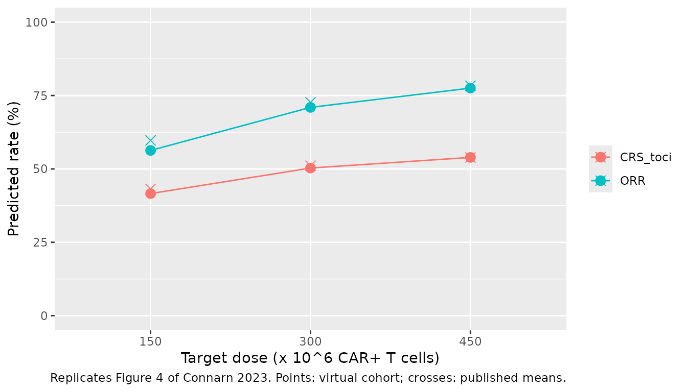
Figure 3: exposure-response curves
grid <- seq(11, 18, by = 0.05)
gp <- predict_all(grid)
curves <- bind_rows(
  data.frame(panel = "(a) ORR", lnauc = grid, p = 100 * gp$orr),
  data.frame(panel = "(b) CRR, M-protein <= 10 g/L", lnauc = grid, p = 100 * gp$cr_lo),
  data.frame(panel = "(b) CRR, M-protein > 10 g/L", lnauc = grid, p = 100 * gp$cr_hi),
  data.frame(panel = "(c) CRS requiring tocilizumab", lnauc = grid, p = 100 * gp$toci),
  data.frame(panel = "(d) CRS requiring steroids", lnauc = grid, p = 100 * gp$ster)
) |>
  mutate(facet = sub(",.*", "", panel))

# Observed rates per log(AUC0-28) quartile (counts printed in Figure 3; the
# quartile medians are digitised).
q_med <- c(13.4, 14.6, 15.4, 16.3)
observed <- data.frame(
  facet = rep(c("(a) ORR", "(b) CRR", "(c) CRS requiring tocilizumab", "(d) CRS requiring steroids"), each = 4),
  lnauc = rep(q_med, 4),
  x = c(10, 25, 29, 29, 3, 11, 13, 14, 8, 20, 18, 19, 1, 3, 7, 7),
  n = rep(c(32, 31, 31, 31), 4)
) |>
  mutate(p = 100 * x / n)

ggplot(curves, aes(lnauc, p)) +
  geom_line(aes(linetype = panel)) +
  geom_point(data = observed) +
  facet_wrap(~facet) +
  coord_cartesian(ylim = c(0, 100)) +
  labs(
    x = "log(AUC0-28)", y = "Response or event rate (%)", linetype = NULL,
    caption = "Replicates Figure 3 of Connarn 2023 (final models; ORR averaged over 41% female)."
  ) +
  theme(legend.position = "bottom") +
  guides(linetype = guide_legend(ncol = 2))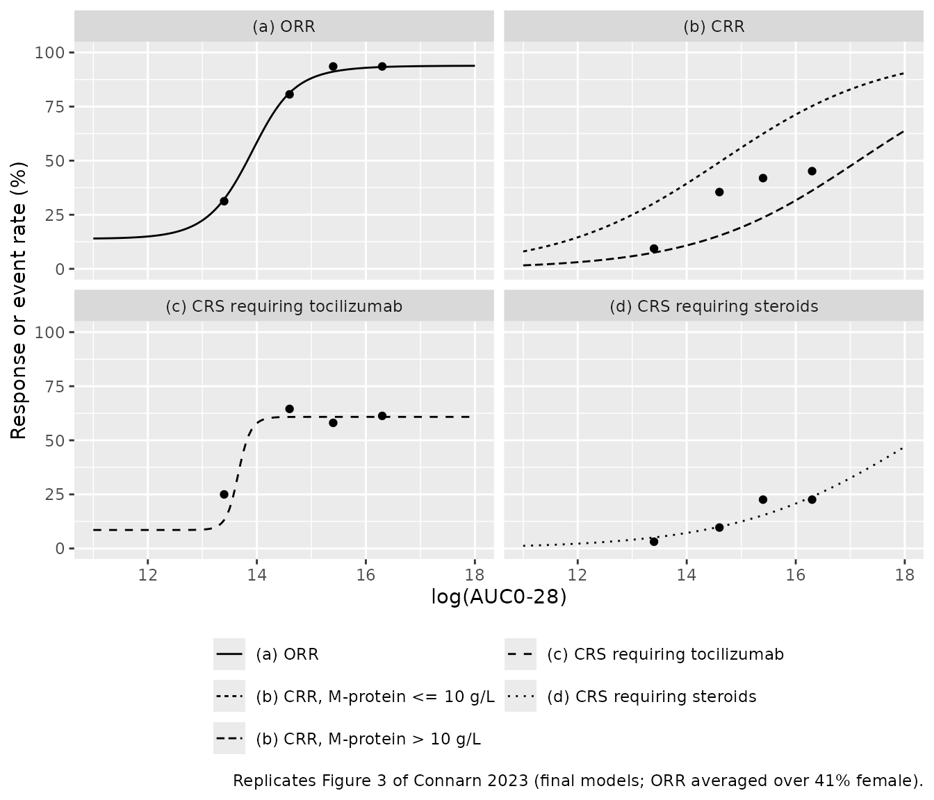
Assumptions and deviations
- ‘Log(EC50)’ and ‘H’ are log-scale estimates. The Figure 3 tables print ‘Log(EC50)’ and ‘H’ for the sigmoid Emax models. The model files take EC50 = exp(Log(EC50)) and Hill = exp(H), both on the log(AUC0-28) axis. Gate 1 shows that only this reading reproduces the plotted curves of Figures 3a and 3c (RMSE about 1 percentage point). The literal reading, H applied as printed, misses by more than 10 points and cannot produce the flat 8.5% floor of the CRS-requiring-tocilizumab curve. Gate 3 shows it also misses the published dose-response rates.
-
Exposure units and log base. The paper
natural-log-transformed AUC0-28 for every exposure-response evaluation.
AUC_IDECELmust be supplied in day*copies/ug, untransformed; each model takeslog()itself. - Female fraction. Connarn 2023 does not report the sex split. The ORR curve in Figure 3a is a population average, and its plateaus fix the female fraction at about 0.41. That value is used for the population-averaged ORR here; it is not a model parameter.
-
M-protein fraction. The fraction of patients with
baseline serum M-protein above 10 g/L is not reported. It was
back-solved from the observed CRR (Gate 2) and is not a model parameter.
The CRR model takes the continuous
MCPROTin g/L and dichotomises it at 10 g/L internally, soMCPROT = 10falls in the reference (<= 10 g/L) group, as in the paper. - Virtual cohort. Individual AUC0-28 values are not published. The cohort is reconstructed from the digitised per-dose medians and 90% ranges of Figure 3, with a split normal distribution in log(AUC0-28). Gates 2 and 3 therefore have tolerances of 6-8 percentage points rather than exact agreement.
- Residual error. The paper fits a Bernoulli likelihood with no between-subject variability and no residual error. Each model carries a fixed additive residual SD of 0.001 on the probability so that rxode2 has an error model to attach; it is not a published quantity.
- Separately fitted end points. ORR and CRR were fitted independently and are not constrained to stay ordered. At very low exposure a male patient’s predicted ORR (about 6%) can fall below the predicted CRR of a patient with M-protein <= 10 g/L (about 8% at log(AUC0-28) = 11). Use each model for its own end point.
- Not modelled. Grade 3 or higher CRS, investigator-identified neurotoxicity and cytopenias showed no exposure-response relationship (Figure S1) and have no model. Connarn 2023 also reports observed rates from the phase I CRB-401 study (Table S1, Figure S2) as an external comparison; they are not fitted by these models. The CRS-requiring-tocilizumab rates in CRB-401 (11.1% and 36.8%) were well below the KarMMa-based predictions.
- No NCA. These are static exposure-response models with no concentration-time output, so there is no PKNCA section; the exposure itself is the noncompartmental AUC0-28 computed by the authors.