MG1113 anti-TFPI antibody two-target TMDD across species (Kwak 2025)

Model and source

Kwak 2025 refines a target-mediated drug disposition (TMDD) model for MG1113, a humanized IgG4 antibody against the Kunitz-type protease inhibitor 2 (K2) domain of tissue factor pathway inhibitor (TFPI), in development for hemophilia. The refinement over the earlier Kwak 2021 model is threefold: both TFPI pools are represented explicitly (soluble TFPI-alpha and the far more abundant membrane-bound TFPI), the empirical feedback compartment used previously to generate the sTFPI-alpha rebound is replaced by a mechanistic one, and a transit compartment is added for delayed subcutaneous absorption.

The paper contributes three model files – one fit and two allometric projections:

Model	Species	Provenance
Kwak_2025_mg1113_monkey	cynomolgus monkey	Fitted to monkey data by the Cluster Gauss-Newton Method (Table 1, rank 1)
Kwak_2025_mg1113_rabbit	rabbit	Allometric projection of the monkey fit; externally validated (Table 3, Figure 3)
Kwak_2025_mg1113_human	human	Allometric projection of the monkey fit; not validated (Table 3, Figure 4)

• Article: https://doi.org/10.3389/fphar.2025.1745702
• Supplement (model equations, Table S1-S4): https://www.frontiersin.org/articles/10.3389/fphar.2025.1745702/full#supplementary-material

models <- list(
  monkey = rxode2::rxode(readModelDb("Kwak_2025_mg1113_monkey")),
  rabbit = rxode2::rxode(readModelDb("Kwak_2025_mg1113_rabbit")),
  human  = rxode2::rxode(readModelDb("Kwak_2025_mg1113_human"))
)
cat(models$monkey$description)
#> Preclinical (cynomolgus monkey). QSP (full TMDD). Refined two-target target-mediated drug disposition model for MG1113, a humanized anti-tissue-factor-pathway-inhibitor (anti-TFPI) IgG4 antibody, describing explicit bimolecular binding to BOTH soluble TFPI-alpha (sTFPI-alpha) and membrane-bound TFPI (mTFPI) in a two-compartment PK framework, with zero-order synthesis / first-order degradation turnover of each target, first-order elimination of each drug-target complex, and a single transit compartment for delayed subcutaneous absorption. Parameters fitted to monkey MG1113 and sTFPI-alpha plasma profiles by the Cluster Gauss-Newton Method (rank 1 accepted parameter set, Kwak 2025 Table 1).

Population

The structural model was fitted to previously published plasma MG1113 and sTFPI-alpha profiles from cynomolgus monkeys (Kwak 2025 section 2.1, reanalysing Kwak 2021). Monkeys received a single intravenous or subcutaneous dose of MG1113 at 2.5, 5.0 or 10.0 mg/kg (17.2, 34.4 or 68.8 nmol/kg), with n = 1-3 per dose/route group. Individual body weights were unavailable, so a representative 3.5 kg was used throughout and doses were converted to 60.2, 120.4 and 240.8 nmol per animal. Both analytes were measured by ELISAs detecting the free forms, and concentrations were converted to molar units using molecular weights of 145.36 kDa (MG1113) and 35 kDa (sTFPI-alpha).

The rabbit cohort (male, 2-3 months, 2.5 kg representative weight) received single i.v. doses of 2.75, 17.2 or 34.4 nmol/kg or single s.c. doses of 17.2, 34.4, 68.8 or 137.6 nmol/kg, n = 2-10 per group. These data were used only to evaluate the allometric projection, never to fit it.

No human MG1113 data were available to the authors, so the human file is a pure forward prediction under the phase I regimens of NCT03855696 (s.c. 0.5, 1.7 and 3.3 mg/kg; i.v. 3.3 mg/kg).

The same information is available programmatically via each model’s population metadata, e.g. readModelDb("Kwak_2025_mg1113_monkey")()$population.

tibble::tibble(
  Model   = names(models),
  Species = vapply(models, function(m) m$population$species, character(1)),
  Dosing  = vapply(models, function(m) m$population$dose_range, character(1))
) |>
  knitr::kable(caption = "Study populations behind each of the three model files.")

Study populations behind each of the three model files.

Model	Species	Dosing
monkey	cynomolgus monkey (Macaca fascicularis)	Single i.v. or s.c. MG1113 at 2.5, 5.0 or 10.0 mg/kg (17.2, 34.4 or 68.8 nmol/kg), i.e. 60.2, 120.4 or 240.8 nmol per 3.5 kg monkey; n = 1-3 per dose/route group
rabbit	rabbit	Single i.v. at 2.75, 17.2 or 34.4 nmol/kg; single s.c. at 17.2, 34.4, 68.8 or 137.6 nmol/kg; n = 2-10 per group
human	human	Simulated single and weekly (Q7d) s.c. doses of 0.5, 1.7 and 3.3 mg/kg and i.v. doses of 3.3 mg/kg (3.44, 11.7 and 22.7 nmol/kg), matching the phase I trial NCT03855696

Model structure

All three files share one structure (Kwak 2025 Figure 1; equations in Supplementary Material section 4). Writing C2 for the free MG1113 concentration in the central compartment:

• Absorption (s.c. only). The depot empties at k01 into a transit compartment, at k02 directly into plasma, and is lost at kloss. The transit compartment feeds plasma at k12.
• Disposition. Two-compartment distribution with inter-compartmental clearance CLD between volumes V2 and V3; first-order elimination of free drug at kel,MG1113.
• Two-target TMDD. MG1113 binds free sTFPI-alpha and free mTFPI with a common association constant kon; koff = KD * kon with KD fixed from the in-vitro measurement. Each target turns over with zero-order synthesis and first-order degradation, and each drug-target complex is eliminated by its own first-order constant (kel,CS and kel,CM).

Two structural notes on the encoding:

1. The paper writes its central and peripheral ODEs on concentration; the model files carry those two states as amounts instead, so that a dose can land on central (i.v.) or depot (s.c.) through an ordinary rxode2 event table. Each ODE is the paper’s equation multiplied through by its compartment volume, so the two forms are identical. The four TFPI-species states (stfpi, mtfpi, astfpi, amtfpi) remain concentrations in nM, exactly as the paper writes them.
2. Neither synthesis rate is a free parameter: both are pinned by the steady-state balance at the reported baseline, ksyn = kdeg * baseline (Supplementary Material section 4, “Related equations”). Likewise koff is pinned by KD.

Source trace

Per-parameter provenance is recorded as an in-file comment beside each ini() entry. Collected here for review:

Equation / parameter	Monkey value	Source location
KD	0.04665 nM (fixed)	Table 1, “Fixed parameter” block (from Kwak 2020)
kon	28.50 1/(nM*day)	Table 1, rank 1
koff = KD * kon	derived	Suppl. Material section 4, “Related equations”
lq (CLD)	0.1454 L/day	Table 1, rank 1
lvc (V2)	0.1112 L	Table 1, rank 1
lvp (V3)	0.1346 L	Table 1, rank 1
k_depot_transit1 (k01)	20.32 /day	Table 1, rank 1
k_depot_central (k02)	8.859e-8 /day	Table 1, rank 1
k_transit1_central (k12)	0.4033 /day	Table 1, rank 1
kloss	3.149e-7 /day	Table 1, rank 1
lkel (kel,MG1113)	0.4543 /day	Table 1, rank 1
kdegs (kdeg,s)	75.50 /day	Table 1, rank 1
kdegm (kdeg,m)	1.150 /day	Table 1, rank 1
kints (kel,CS)	0.3094 /day	Table 1, rank 1
kintm (kel,CM)	0.006851 /day	Table 1, rank 1
stfpi_b	0.9456 nM	Table 1, rank 1
mtfpi_b	12.04 nM	Table 1, rank 1
ksyn = kdeg * baseline	derived	Suppl. Material section 4, “Related equations”
all d/dt(...) equations	n/a	Suppl. Material section 4, “Model equations”
rabbit / human parameter columns	see Table 3	Table 3; allometry per section 2.6

Simulation helpers

Every model here is a typical-value deterministic simulator: the CGNM fit targeted the mean observed profiles, so the paper reports no inter-individual variability and no residual-error model, and none is encoded. There is therefore no cohort to draw and no VPC to build – one subject per arm reproduces the published curves exactly, and every assertion below is on a deterministic quantity, so tight bounds are appropriate.

MW_MG1113 <- 145360                      # g/mol, Kwak 2025 section 2.1
nM_to_ugmL <- MW_MG1113 * 1e-9 * 1e3     # 1 nM = 0.14536 ug/mL

# A time grid dense enough to resolve the steep early distribution phase (an
# under-resolved grid understates AUC by several percent; see pattern 11 of
# the known-vignette-failure-patterns reference).
obs_grid <- function(tmax) {
  sort(unique(c(
    seq(0, 1, by = 0.002),
    seq(1, 10, by = 0.01),
    seq(10, tmax, by = 0.05)
  )))
}

# Build an explicit event table. Observation rows carry cmt = "central" -- an
# ODE STATE, never the observable name "Cc" (that would auto-inject a cmt()
# slot and renumber every compartment).
make_events <- function(amt, route, tmax, ii = NULL, addl = 0L, id = 1L) {
  dose_cmt <- if (route == "iv") "central" else "depot"
  dose_times <- if (is.null(ii)) 0 else seq(0, by = ii, length.out = addl + 1L)
  dplyr::bind_rows(
    tibble::tibble(id = id, time = dose_times, amt = amt, evid = 1L, cmt = dose_cmt),
    tibble::tibble(id = id, time = obs_grid(tmax), amt = NA_real_, evid = 0L, cmt = "central")
  ) |>
    dplyr::arrange(time, dplyr::desc(evid))
}

solve_arm <- function(model, events, keep = character()) {
  # useLinCmt = FALSE: rxode2's automatic ODE->linCmt conversion corrupts the
  # observable mapping for multi-output multi-state models.
  out <- rxode2::rxSolve(model, events = events, keep = keep, useLinCmt = FALSE) |>
    as.data.frame()
  if (is.null(out$id)) out$id <- 1L
  out
}

# Trapezoidal AUC on a solved arm.
auc_of <- function(df, col, from = 0, to = Inf) {
  d <- df[df$time >= from & df$time <= to, ]
  d <- d[order(d$time), ]
  sum(diff(d$time) * (utils::head(d[[col]], -1) + utils::tail(d[[col]], -1)) / 2)
}

Structural check 1: the undosed system sits exactly at baseline

ksyn = kdeg * baseline should hold each target perfectly flat in the absence of drug. This is a deterministic identity, so the tolerance is machine precision, not a tuned bound – it goes red on any mis-transcribed baseline, degradation rate or synthesis expression.

ss <- lapply(names(models), function(sp) {
  m  <- models[[sp]]
  ev <- tibble::tibble(id = 1L, time = seq(0, 60, by = 0.25),
                       amt = NA_real_, evid = 0L, cmt = "central")
  s  <- solve_arm(m, ev)
  b  <- m$theta
  tibble::tibble(
    Species          = sp,
    `sTFPI-a base (nM)` = unname(b[["stfpi_b"]]),
    `max |dev|`      = max(abs(s$sTFPI - unname(b[["stfpi_b"]]))),
    `mTFPI base (nM)` = unname(b[["mtfpi_b"]]),
    `max |dev| mTFPI` = max(abs(s$mtfpi - unname(b[["mtfpi_b"]])))
  )
}) |> dplyr::bind_rows()

knitr::kable(ss, digits = 12,
             caption = "Undosed steady state: both targets hold their baseline exactly.")

Undosed steady state: both targets hold their baseline exactly.

Species	sTFPI-a base (nM)	max |dev|	mTFPI base (nM)	max |dev| mTFPI
monkey	0.9456	0	12.04	0
rabbit	1.1140	0	14.19	0
human	2.3000	0	29.11	0

stopifnot(all(ss$`max |dev|` < 1e-6), all(ss$`max |dev| mTFPI` < 1e-6))

Structural check 2: the allometric scaling reproduces Table 3

Table 3 is the monkey rank 1 column scaled to 2.5 kg (rabbit) and 70 kg (human) with exponents 0.75 for CLD, -0.25 for every rate constant and 1.0 for the volumes (Kwak 2025 section 2.6). Recomputing that scaling from the monkey file and comparing against the values actually encoded in the rabbit and human files checks the whole Table 3 transcription in one step.

BW <- c(monkey = 3.5, rabbit = 2.5, human = 70.0)   # Table 3
expo <- c(lq = 0.75, lvc = 1.0, lvp = 1.0,
          k_depot_transit1 = -0.25, k_depot_central = -0.25,
          k_transit1_central = -0.25, lkel = -0.25,
          kdegs = -0.25, kdegm = -0.25, kints = -0.25, kintm = -0.25,
          kloss = -0.25)
# Parameters held on the log scale in ini() must be scaled on the linear scale.
log_scale <- c("lq", "lvc", "lvp", "lkel")

theta_lin <- function(m) {
  th <- m$theta
  for (p in log_scale) th[[p]] <- exp(th[[p]])
  th
}
mk <- theta_lin(models$monkey)

allo <- lapply(c("rabbit", "human"), function(sp) {
  tgt <- theta_lin(models[[sp]])
  ratio <- BW[[sp]] / BW[["monkey"]]
  tibble::tibble(
    Species   = sp,
    Parameter = names(expo),
    Expected  = unname(mk[names(expo)]) * ratio^unname(expo),
    Encoded   = unname(tgt[names(expo)])
  )
}) |>
  dplyr::bind_rows() |>
  dplyr::mutate(`% diff` = 100 * (Encoded - Expected) / Expected)

allo |>
  dplyr::mutate(dplyr::across(c(Expected, Encoded), ~ signif(.x, 4)),
                `% diff` = round(`% diff`, 2)) |>
  knitr::kable(caption = paste(
    "Table 3 check: each rabbit / human value recomputed from the monkey fit",
    "and the paper's allometric exponents, vs the value encoded in the file."))

Table 3 check: each rabbit / human value recomputed from the monkey fit and the paper’s allometric exponents, vs the value encoded in the file.

Species	Parameter	Expected	Encoded	% diff
rabbit	lq	1.130e-01	1.130e-01	0.03
rabbit	lvc	7.943e-02	7.944e-02	0.01
rabbit	lvp	9.614e-02	9.615e-02	0.01
rabbit	k_depot_transit1	2.210e+01	2.210e+01	-0.01
rabbit	k_depot_central	1.000e-07	1.000e-07	0.01
rabbit	k_transit1_central	4.387e-01	4.387e-01	0.00
rabbit	lkel	4.942e-01	4.942e-01	0.01
rabbit	kdegs	8.213e+01	8.213e+01	0.01
rabbit	kdegm	1.251e+00	1.251e+00	0.01
rabbit	kints	3.366e-01	3.366e-01	0.01
rabbit	kintm	7.452e-03	7.452e-03	0.00
rabbit	kloss	3.000e-07	3.000e-07	-0.01
human	lq	1.375e+00	1.375e+00	-0.01
human	lvc	2.224e+00	2.224e+00	0.00
human	lvp	2.692e+00	2.692e+00	0.00
human	k_depot_transit1	9.609e+00	9.609e+00	0.00
human	k_depot_central	0.000e+00	0.000e+00	0.00
human	k_transit1_central	1.907e-01	1.907e-01	0.00
human	lkel	2.148e-01	2.148e-01	-0.01
human	kdegs	3.570e+01	3.570e+01	0.00
human	kdegm	5.438e-01	5.440e-01	0.04
human	kints	1.463e-01	1.463e-01	0.00
human	kintm	3.240e-03	3.240e-03	0.01
human	kloss	1.000e-07	1.000e-07	0.00

# The paper rounds Table 3 to 4 significant figures, so exact agreement is not
# expected; anything beyond ~0.5% would mean a mis-transcribed column.
stopifnot(max(abs(allo$`% diff`)) < 0.5)

The two target baselines are deliberately excluded from that check: they are not allometrically scaled. stfpi_b is a per-species literature value (0.9456 nM fitted in monkeys, 1.114 nM in rabbits from Kwak 2020, 2.3 nM in humans from Kwak 2021) and mtfpi_b follows from the monkey mTFPI:sTFPI-alpha ratio of 12.7 (Supplementary Material item 7).

tibble::tibble(
  Species = names(models),
  `sTFPI-a base (nM)` = vapply(models, function(m) unname(m$theta[["stfpi_b"]]), numeric(1)),
  `mTFPI base (nM)`   = vapply(models, function(m) unname(m$theta[["mtfpi_b"]]), numeric(1))
) |>
  dplyr::mutate(Ratio = round(`mTFPI base (nM)` / `sTFPI-a base (nM)`, 2)) |>
  knitr::kable(caption = "Target baselines are per-species literature values, not allometric projections.")

Target baselines are per-species literature values, not allometric projections.

Species	sTFPI-a base (nM)	mTFPI base (nM)	Ratio
monkey	0.9456	12.04	12.73
rabbit	1.1140	14.19	12.74
human	2.3000	29.11	12.66

Replicating Figure 2: monkey MG1113 and sTFPI-alpha

monkey_doses <- c("17.2 nmol/kg" = 60.2, "34.4 nmol/kg" = 120.4, "68.8 nmol/kg" = 240.8)

monkey_sim <- do.call(dplyr::bind_rows, lapply(c("iv", "sc"), function(rt) {
  do.call(dplyr::bind_rows, lapply(names(monkey_doses), function(dl) {
    solve_arm(models$monkey, make_events(monkey_doses[[dl]], rt, tmax = 28)) |>
      dplyr::mutate(route = toupper(rt), dose = dl)
  }))
}))

monkey_sim |>
  dplyr::filter(time > 0) |>
  tidyr::pivot_longer(c(Cc, sTFPI), names_to = "analyte", values_to = "conc") |>
  dplyr::mutate(analyte = dplyr::recode(analyte, Cc = "MG1113", sTFPI = "sTFPI-alpha")) |>
  ggplot(aes(time, conc, colour = dose)) +
  geom_line(linewidth = 0.7) +
  facet_grid(analyte ~ route, scales = "free_y") +
  scale_y_log10() +
  labs(x = "Time (day)", y = "Plasma concentration (nM)", colour = "Dose",
       title = "Figure 2 - monkey MG1113 and sTFPI-alpha profiles",
       caption = "Replicates Figure 2 of Kwak 2025 (rank 1 parameter set).") +
  theme_bw()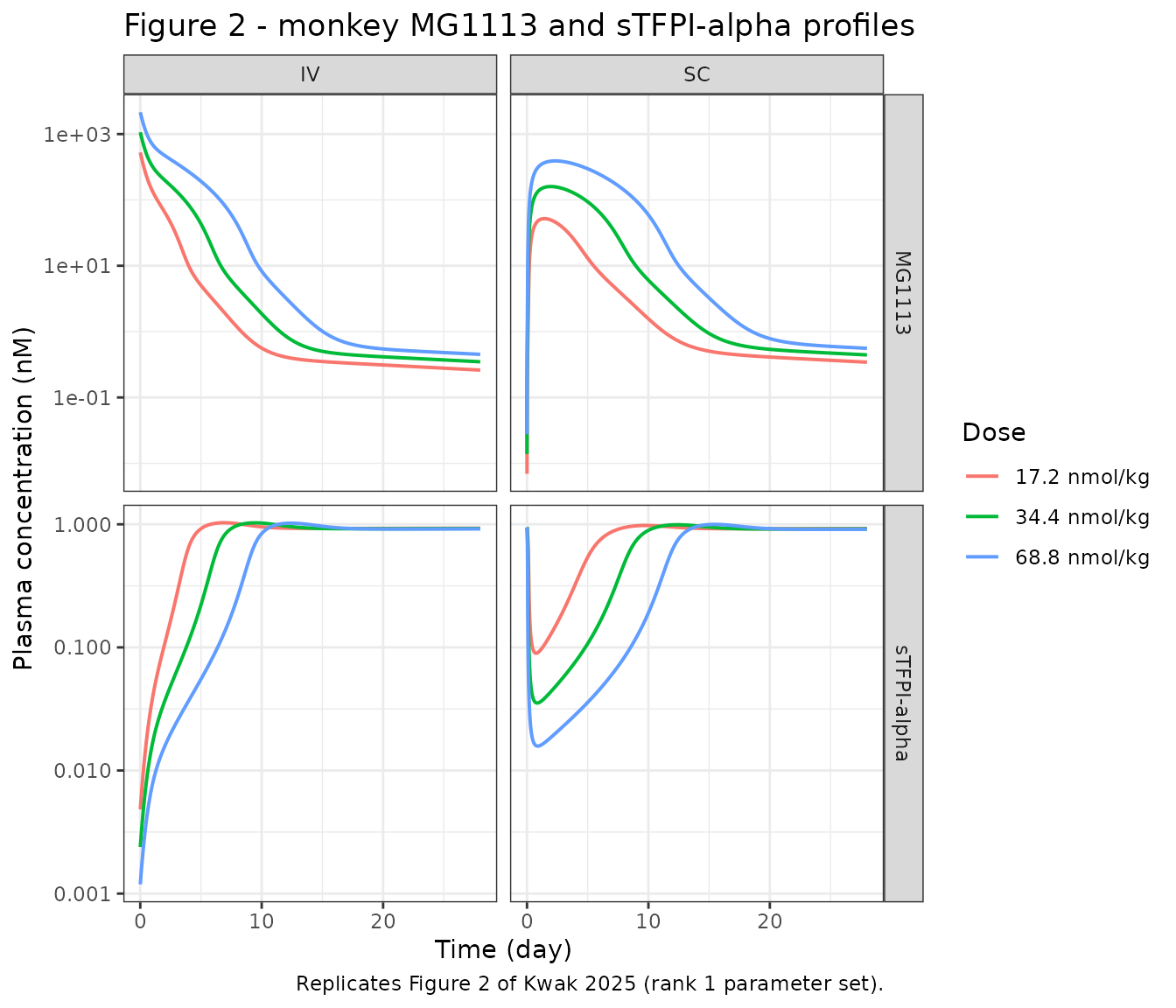

The mechanistic point of the refinement is the sTFPI-alpha rebound: Aston 2014/2017 show a rebound arises when the complex internalisation rate is slower than both the free-drug elimination rate and the free-target degradation rate. The monkey fit satisfies exactly that ordering, and the simulated profile overshoots baseline as a result.

b   <- models$monkey$theta
ord <- c(`kel,CS (complex)` = unname(b[["kints"]]),
         `kel,MG1113 (free drug)` = exp(unname(b[["lkel"]])),
         `kdeg,s (free target)` = unname(b[["kdegs"]]))

hi  <- monkey_sim |> dplyr::filter(route == "IV", dose == "68.8 nmol/kg")
nadir_t <- hi$time[which.min(hi$sTFPI)]
peak    <- max(hi$sTFPI[hi$time > nadir_t])
base    <- unname(b[["stfpi_b"]])

knitr::kable(
  tibble::tibble(Quantity = names(ord), `Value (1/day)` = signif(unname(ord), 4)),
  caption = "Aston rebound condition: kel,CS must be below BOTH of the other two rates.")

Aston rebound condition: kel,CS must be below BOTH of the other two rates.

Quantity	Value (1/day)
kel,CS (complex)	0.3094
kel,MG1113 (free drug)	0.4543
kdeg,s (free target)	75.5000

cat(sprintf(
  "IV 68.8 nmol/kg: baseline %.4f nM, nadir %.4g nM at day %.2f, post-nadir peak %.4f nM (%.1f%% of baseline).\n",
  base, min(hi$sTFPI), nadir_t, peak, 100 * peak / base))
#> IV 68.8 nmol/kg: baseline 0.9456 nM, nadir 0.00119 nM at day 0.00, post-nadir peak 1.0214 nM (108.0% of baseline).

stopifnot(
  # The rebound condition the paper argues from (Discussion, section 4).
  ord[["kel,CS (complex)"]] < ord[["kel,MG1113 (free drug)"]],
  ord[["kel,CS (complex)"]] < ord[["kdeg,s (free target)"]],
  # ... and the rebound it predicts: sTFPI-alpha overshoots its own baseline.
  peak > base
)

Replicating Figure 3: the rabbit projection

rabbit_arms <- tibble::tribble(
  ~route, ~label,           ~nmol_per_kg,
  "iv",   "IV 2.75",        2.75,
  "iv",   "IV 17.2",        17.2,
  "iv",   "IV 34.4",        34.4,
  "sc",   "SC 17.2",        17.2,
  "sc",   "SC 34.4",        34.4,
  "sc",   "SC 68.8",        68.8,
  "sc",   "SC 137.6",       137.6
) |>
  dplyr::mutate(amt = nmol_per_kg * 2.5)   # 2.5 kg representative rabbit

rabbit_sim <- do.call(dplyr::bind_rows, lapply(seq_len(nrow(rabbit_arms)), function(i) {
  solve_arm(models$rabbit, make_events(rabbit_arms$amt[i], rabbit_arms$route[i], tmax = 21)) |>
    dplyr::mutate(route = toupper(rabbit_arms$route[i]), arm = rabbit_arms$label[i])
}))

rabbit_sim |>
  dplyr::filter(time > 0) |>
  tidyr::pivot_longer(c(Cc, sTFPI), names_to = "analyte", values_to = "conc") |>
  dplyr::mutate(analyte = dplyr::recode(analyte, Cc = "MG1113", sTFPI = "sTFPI-alpha")) |>
  ggplot(aes(time, conc, colour = arm)) +
  geom_line(linewidth = 0.7) +
  facet_wrap(~ analyte, scales = "free_y") +
  scale_y_log10() +
  labs(x = "Time (day)", y = "Plasma concentration (nM)", colour = "Arm",
       title = "Figure 3 - rabbit projection under the observed dosing arms",
       caption = "Replicates Figure 3 of Kwak 2025. Parameters are allometric predictions, not a rabbit fit.") +
  theme_bw()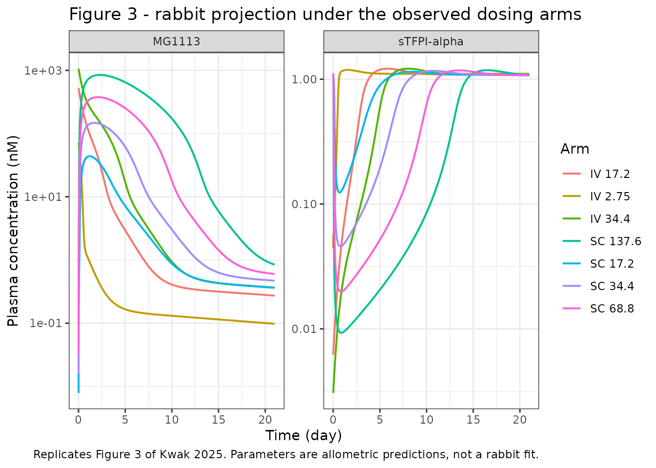

The paper compares these predictions with observed rabbit data and reports absolute average fold errors of 1.5-1.9 in the high-dose groups but 2.8-4.2 in the low-dose groups, where the model over-predicts and misses a rapid decline (section 3.2). The rabbit observations themselves are not published as a table, so that comparison cannot be reproduced numerically here; it is recorded as a known limitation of the rabbit file rather than reproduced.

Replicating Figure 4: the human projection

human_doses_mgkg <- c("0.5 mg/kg" = 0.5, "1.7 mg/kg" = 1.7, "3.3 mg/kg" = 3.3)
# Kwak 2025 section 3.3: 0.5, 1.7, 3.3 mg/kg = 3.44, 11.7, 22.7 nmol/kg
human_doses_nmol <- c("0.5 mg/kg" = 3.44, "1.7 mg/kg" = 11.7, "3.3 mg/kg" = 22.7) * 70

human_single <- do.call(dplyr::bind_rows, lapply(c("iv", "sc"), function(rt) {
  do.call(dplyr::bind_rows, lapply(names(human_doses_nmol), function(dl) {
    solve_arm(models$human, make_events(human_doses_nmol[[dl]], rt, tmax = 30)) |>
      dplyr::mutate(route = toupper(rt), dose = dl)
  }))
}))

human_q7d <- do.call(dplyr::bind_rows, lapply(c("iv", "sc"), function(rt) {
  do.call(dplyr::bind_rows, lapply(names(human_doses_nmol), function(dl) {
    solve_arm(models$human,
              make_events(human_doses_nmol[[dl]], rt, tmax = 56, ii = 7, addl = 7L)) |>
      dplyr::mutate(route = toupper(rt), dose = dl)
  }))
}))

stfpi_base_human <- unname(models$human$theta[["stfpi_b"]])

dplyr::bind_rows(
  dplyr::mutate(human_single, panel = "Single dose"),
  dplyr::mutate(human_q7d,    panel = "Q7d x 8")
) |>
  dplyr::filter(time > 0) |>
  ggplot(aes(time, sTFPI, colour = dose)) +
  geom_line(linewidth = 0.7) +
  geom_hline(yintercept = 0.25 * stfpi_base_human, linetype = "dotted") +
  facet_grid(panel ~ route, scales = "free_x") +
  labs(x = "Time (day)", y = "Plasma sTFPI-alpha (nM)", colour = "Dose",
       title = "Figure 4 - predicted human sTFPI-alpha suppression",
       caption = paste("Replicates Figure 4B/4D of Kwak 2025. Dotted line = 25% of the",
                       "2.3 nM baseline, the efficacy-associated target.")) +
  theme_bw()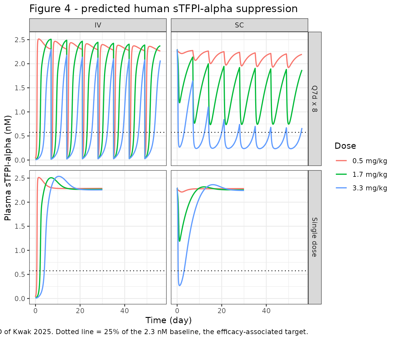

PKNCA validation against Supplementary Table S3

Supplementary Table S3 tabulates the model’s own predicted human AUC_0-30days for all six single-dose arms, in day*ug/mL. Because the integration window is stated exactly (0 to 30 days), this is an exact validation target rather than an approximate one: a correct re-implementation must reproduce all six numbers. Any error in an ODE term, a parameter value, the molar dose conversion or the nM-to-ug/mL conversion moves them.

sim_nca <- human_single |>
  dplyr::mutate(arm = paste(route, dose)) |>
  dplyr::filter(!is.na(Cc)) |>
  dplyr::select(id, time, Cc, arm)

# Guarantee a time = 0 row per arm so PKNCA can anchor AUC0-30. IDs are shared
# across arms here (one deterministic subject per arm), so the arm label -- not
# id -- is the grouping that matters; give each arm its own id to be safe.
sim_nca <- sim_nca |>
  dplyr::mutate(id = as.integer(factor(arm)))

sim_nca <- dplyr::bind_rows(
  sim_nca,
  sim_nca |> dplyr::distinct(id, arm) |> dplyr::mutate(time = 0, Cc = 0)
) |>
  dplyr::distinct(id, arm, time, .keep_all = TRUE) |>
  dplyr::arrange(id, arm, time)

conc_obj <- PKNCA::PKNCAconc(sim_nca, Cc ~ time | arm + id)

dose_df <- human_single |>
  dplyr::mutate(arm = paste(route, dose)) |>
  dplyr::distinct(arm, dose, route) |>
  dplyr::mutate(id = as.integer(factor(arm)), time = 0,
                amt = unname(human_doses_nmol[dose]))

dose_obj <- PKNCA::PKNCAdose(dose_df, amt ~ time | arm + id)
#> Found column named route, using it for the attribute of the same name.

intervals <- data.frame(
  start = 0, end = 30,
  auclast = TRUE, cmax = TRUE, tmax = TRUE
)

nca_res <- PKNCA::pk.nca(PKNCA::PKNCAdata(conc_obj, dose_obj, intervals = intervals))

# Supplementary Table S3, single-administration block (day*ug/mL), converted to
# the model's native day*nM so the comparison stays in the units the model emits.
published <- tibble::tribble(
  ~arm,          ~auclast_ugmL,
  "IV 0.5 mg/kg",   4.018,
  "IV 1.7 mg/kg",  40.16,
  "IV 3.3 mg/kg", 119.4,
  "SC 0.5 mg/kg",   0.5931,
  "SC 1.7 mg/kg",   4.005,
  "SC 3.3 mg/kg",  18.52
) |>
  dplyr::mutate(auclast = auclast_ugmL / nM_to_ugmL) |>
  dplyr::select(arm, auclast)

cmp <- nlmixr2lib::ncaComparisonTable(
  simulated = nca_res,
  reference = published,
  by        = "arm",
  params    = "auclast",
  units     = c(auclast = "day*nM"),
  tolerance_pct = 20
)

knitr::kable(
  cmp,
  caption = paste("Simulated vs Kwak 2025 Supplementary Table S3 AUC(0-30 days).",
                  "* marks a >20% difference."),
  align = c("l", "l", "r", "r", "r")
)

Simulated vs Kwak 2025 Supplementary Table S3 AUC(0-30 days). * marks a >20% difference.

NCA parameter	arm	Reference	Simulated	% diff
AUClast (day*nM)	IV 0.5 mg/kg	27.6	27.4	-0.8%
AUClast (day*nM)	IV 1.7 mg/kg	276	276	-0.3%
AUClast (day*nM)	IV 3.3 mg/kg	821	819	-0.3%
AUClast (day*nM)	SC 0.5 mg/kg	4.08	4.07	-0.1%
AUClast (day*nM)	SC 1.7 mg/kg	27.6	27.4	-0.4%
AUClast (day*nM)	SC 3.3 mg/kg	127	126	-1.2%

# Independent numeric gate on the same six values (the table above is for the
# reader; this is what fails the render). Deterministic model, exactly specified
# window -- so the only slack needed is trapezoidal-integration error on the
# steep distribution phase plus the paper's 4-significant-figure rounding.
gate <- human_single |>
  dplyr::mutate(arm = paste(route, dose)) |>
  dplyr::group_by(arm) |>
  dplyr::group_modify(~ tibble::tibble(
    sim_ugmL = auc_of(.x, "Cc", 0, 30) * nM_to_ugmL)) |>
  dplyr::ungroup() |>
  dplyr::left_join(
    published |> dplyr::mutate(paper_ugmL = auclast * nM_to_ugmL) |>
      dplyr::select(arm, paper_ugmL),
    by = "arm") |>
  dplyr::mutate(`% diff` = 100 * (sim_ugmL - paper_ugmL) / paper_ugmL)

gate |>
  dplyr::mutate(dplyr::across(c(sim_ugmL, paper_ugmL), ~ signif(.x, 4)),
                `% diff` = round(`% diff`, 2)) |>
  dplyr::rename("Arm" = arm,
                "Simulated AUC0-30d (day*ug/mL)" = sim_ugmL,
                "Table S3 (day*ug/mL)" = paper_ugmL) |>
  knitr::kable(caption = "AUC(0-30 days): simulation vs the paper's own predicted values.")

AUC(0-30 days): simulation vs the paper’s own predicted values.

Arm	Simulated AUC0-30d (day*ug/mL)	Table S3 (day*ug/mL)	% diff
IV 0.5 mg/kg	3.9860	4.0180	-0.79
IV 1.7 mg/kg	40.0500	40.1600	-0.27
IV 3.3 mg/kg	119.0000	119.4000	-0.30
SC 0.5 mg/kg	0.5922	0.5931	-0.14
SC 1.7 mg/kg	3.9870	4.0050	-0.45
SC 3.3 mg/kg	18.3000	18.5200	-1.21

# Realised max |% diff| ~1.2% on the grid above. 5% still goes red on a
# mis-transcribed rate constant, volume or dose conversion, all of which move
# these AUCs by tens of percent.
stopifnot(max(abs(gate$`% diff`)) < 5)

The paper also reports that dose-normalised AUC rises more than proportionally with dose, more steeply after s.c. than i.v. dosing – the signature of saturable target binding (section 3.3, Supplementary Table S3).

dn <- gate |>
  tidyr::separate(arm, into = c("route", "dose_mgkg"), sep = " ", extra = "merge") |>
  dplyr::mutate(dose_mgkg = as.numeric(sub(" mg/kg", "", dose_mgkg)),
                dn_auc = paper_ugmL / dose_mgkg) |>
  dplyr::arrange(route, dose_mgkg)

dn |>
  dplyr::mutate(dn_auc = signif(dn_auc, 4)) |>
  dplyr::select(Route = route, `Dose (mg/kg)` = dose_mgkg,
                `Dose-normalised AUC0-30d` = dn_auc) |>
  knitr::kable(caption = "Dose-normalised AUC increases with dose (more-than-proportional exposure).")

Dose-normalised AUC increases with dose (more-than-proportional exposure).

Route	Dose (mg/kg)	Dose-normalised AUC0-30d
IV	0.5	8.036
IV	1.7	23.620
IV	3.3	36.180
SC	0.5	1.186
SC	1.7	2.356
SC	3.3	5.612

fold <- dn |>
  dplyr::group_by(route) |>
  dplyr::summarise(fold = dn_auc[which.max(dose_mgkg)] / dn_auc[which.min(dose_mgkg)],
                   .groups = "drop")
print(fold)
#> # A tibble: 2 × 2
#>   route  fold
#>   <chr> <dbl>
#> 1 IV     4.50
#> 2 SC     4.73

stopifnot(
  # More than dose proportional in BOTH routes ...
  all(fold$fold > 1),
  # ... and more markedly so after s.c. dosing (section 3.3).
  fold$fold[fold$route == "SC"] > fold$fold[fold$route == "IV"]
)

The paper’s dosing conclusions, checked

Section 3.3 makes four specific, deterministic claims about human sTFPI-alpha suppression. Each is evaluated against the simulation.

thresh <- 0.25 * stfpi_base_human

# Rows of one arm, optionally restricted to a time window, sorted by time.
arm_rows <- function(df, dose_label, route_label, from = 0, to = Inf) {
  df |>
    dplyr::filter(dose == dose_label, route == route_label,
                  time >= from, time <= to) |>
    dplyr::arrange(time)
}
# Does the arm ever get below 25% of baseline?
ever_below <- function(...) any(arm_rows(...)$sTFPI < thresh)
# Time (days) spent below 25% of baseline within the window.
dur_below <- function(...) {
  d <- arm_rows(...)
  # Guard against a lookup that silently matches no rows (pattern 10).
  stopifnot(nrow(d) > 1)
  sum(diff(d$time) * utils::head(d$sTFPI < thresh, -1))
}

iv_all   <- vapply(names(human_doses_nmol),
                   function(d) ever_below(human_single, d, "IV"), logical(1))
sc_any   <- vapply(names(human_doses_nmol),
                   function(d) ever_below(human_single, d, "SC"), logical(1))
sc33_dur <- dur_below(human_single, "3.3 mg/kg", "SC")
# Final full dosing interval of the Q7d run (doses at 0..49; interval 49-56).
ss_frac  <- dur_below(human_q7d, "3.3 mg/kg", "SC", from = 49, to = 56) / 7

claims <- tibble::tribble(
  ~Claim, ~Achieved, ~Pass,
  "Single i.v. drives sTFPI-a below 25% of baseline at ALL doses",
  paste(sprintf("%s: %s", names(iv_all), iv_all), collapse = "; "),
  all(iv_all),

  "Single s.c. reaches it ONLY at 3.3 mg/kg",
  paste(sprintf("%s: %s", names(sc_any), sc_any), collapse = "; "),
  identical(unname(sc_any), c(FALSE, FALSE, TRUE)),

  "Single s.c. 3.3 mg/kg holds suppression for ~3 days",
  sprintf("%.2f days", sc33_dur),
  abs(sc33_dur - 3) < 1.5,

  "Q7d s.c. 3.3 mg/kg holds it for the MAJORITY of the steady-state interval",
  sprintf("%.0f%% of the final 7-day interval", 100 * ss_frac),
  ss_frac > 0.5
)

knitr::kable(claims, caption = "Kwak 2025 section 3.3 dosing conclusions, evaluated against the packaged human model.")

Kwak 2025 section 3.3 dosing conclusions, evaluated against the packaged human model.

Claim	Achieved	Pass
Single i.v. drives sTFPI-a below 25% of baseline at ALL doses	0.5 mg/kg: TRUE; 1.7 mg/kg: TRUE; 3.3 mg/kg: TRUE	TRUE
Single s.c. reaches it ONLY at 3.3 mg/kg	0.5 mg/kg: FALSE; 1.7 mg/kg: FALSE; 3.3 mg/kg: TRUE	TRUE
Single s.c. 3.3 mg/kg holds suppression for ~3 days	2.64 days	TRUE
Q7d s.c. 3.3 mg/kg holds it for the MAJORITY of the steady-state interval	92% of the final 7-day interval	TRUE

stopifnot(all(claims$Pass))

Assumptions and deviations

• Publication year. The model files, the vignette basename and the citation use 2025, matching the DOI (10.3389/fphar.2025.1745702), the EuropePMC pubYear, and the PMCID record. The journal’s own suggested-citation block reads “(2026)” because Frontiers first published the article online on 2026-01-07 against a 2025 DOI. No content differs between the two.
• ODEs rewritten from concentration to amount for two states. The paper writes dC2/dt and dC3/dt on concentration; the model files carry central and peripheral1 as amounts (each equation multiplied through by its volume) so that i.v. and s.c. dosing both work through a standard rxode2 event table. This is an algebraically identical restatement, not a modelling change. The four TFPI-species states remain concentrations in nM as published.
• No IIV and no residual error are encoded, because none are reported. CGNM was fitted to the mean observed profiles by least squares; the paper reports no random-effects model of any kind. These files are typical-value deterministic simulators and cannot be used for individual-level VPCs without variability supplied from elsewhere.
• Five parameters are non-identifiable. Approximate profile likelihood (Supplementary Table S1) declares k02, kel,CM, kel,CS, kloss and kon non-identifiable. kon had two local minima; the authors used the first, which is what is encoded. k02 and kloss are retained at their minute rank 1 values rather than set to zero, following the authors’ explicit choice to “maintain a general model applicable to other antibody therapeutics” (section 3.1); Supplementary Table S2 shows fixing them to zero changes the remaining estimates and the minimum SSR negligibly. Do not read these five values as well-determined.
• The rabbit and human files are predictions, not fits. Every parameter in them is wrapped in fixed() for that reason. The rabbit projection was evaluated against observed data and over-predicts the low-dose arms (AAFE 2.8-4.2); the human projection was never validated against any human data, which the authors state explicitly. Treat the human file as a forward prediction under a stated allometric assumption.
• Binding parameters assumed conserved across species. KD and kon are not scaled, on the strength of K2-domain sequence similarity (human vs monkey 96% identity; human vs rabbit 92%). The fitted in-vivo kon (28.5 1/(nM*day)) is roughly 10-fold below the in-vitro value of Kwak 2020; the authors keep the in-vitro KD and let koff follow (section 4).
• Monkey Table 2 AUC(last) is not reproduced numerically. Table 2 compares observed and predicted AUC to the last measurable concentration, but neither the sampling schedule nor the per-arm last measurable time is tabulated in this paper, so the integration window cannot be reconstructed. The exactly specified Supplementary Table S3 AUC(0-30 days) is used as the numeric gate instead.
• Rabbit observed data are not tabulated in the paper (Figure 3 only), so the published AAFE values are recorded above rather than recomputed.
• sTFPI-alpha baseline as a source of variability. The paper explores a 1.3-2.9 nM human baseline by local sensitivity analysis rather than as a fitted covariate; it is recorded in the human file’s covariatesDataExcluded metadata. To reproduce Figure 5, set stfpi_b and rescale mtfpi_b = 12.7 * stfpi_b.
• Supplement provenance. The model equations are in the Supplementary Material (DataSheet1.pdf), retrieved from the EuropePMC supplementary-files endpoint for PMC12819659 and stored alongside the lead PDF. They are not in the main article text.