Midazolam intestinal and hepatic CYP3A metabolism in children (Brussee 2018b)
Source:vignettes/articles/Brussee_2018b_midazolam_children_pbpk.Rmd
Brussee_2018b_midazolam_children_pbpk.RmdModel and source
- Citation: Brussee JM, Yu H, Krekels EHJ, Palic S, Brill MJE, Barrett JS, Rostami-Hodjegan A, de Wildt SN, Knibbe CAJ (2018). Characterization of Intestinal and Hepatic CYP3A-Mediated Metabolism of Midazolam in Children Using a Physiological Population Pharmacokinetic Modelling Approach. Pharm Res 35(9):182. doi:10.1007/s11095-018-2458-6.
- Description: PBPK (semi-physiological; well-stirred liver + Qgut gut wall) population PK model for midazolam and its primary metabolite 1-OH-midazolam in 264 post-operative children 1-18 years of age after a single oral dose. Physiological gut-wall, portal-vein and liver compartments carry the first-pass and systemic CYP3A metabolism for both analytes, and feed empirical central plus two peripheral compartments for midazolam and a single central compartment for 1-OH-midazolam. Tissue volumes, organ blood flows, plasma albumin, hematocrit, intestinal surface area and the blood:plasma ratio are all derived inside the model from body weight, age and sex (height and body surface area are derived first); the only estimated quantities are the whole-organ intrinsic clearances of the gut wall and liver, the inter-compartmental clearances, and their body-weight power exponents. Distribution volumes are fixed from an adult analysis and scaled linearly with body weight. The model runs in molar units, so the fraction of midazolam metabolised to 1-OH-midazolam is 1 with no molecular-weight conversion.
- Article: https://doi.org/10.1007/s11095-018-2458-6
- Supplement (open access, Springer ESM 1): https://doi.org/10.1007/s11095-018-2458-6
Note on the file stem. A different Brussee 2018 midazolam model is
already packaged as Brussee_2018_midazolam_pbpk – that is
doi:10.1002/psp4.12295,
a semi-physiological model in 37 preterm neonates. The
present model is a separate paper (doi:10.1007/s11095-018-2458-6)
in 264 children aged 1-18 years, so it takes the
year-letter suffix 2018b.
Population
Brussee 2018 analysed 865 plasma samples from 264 post-operative children of the Children’s Hospital of Philadelphia (Table SI of the supplement). Children were 1-18 years old (median 7 years) with a median body weight of 27.4 kg (range 9.1-137.6 kg), 148 boys and 116 girls (43.9% female), all American Society of Anesthesiologists physical status class I or II and undergoing surgery. Each received a single pre-operative oral dose of midazolam suspension (median 10 mg, range 3-15 mg). Thirty-one children were densely sampled (median 10 samples, range 8-11) and 233 sparsely sampled (median 2 samples, range 1-3). Both midazolam and its CYP3A-mediated metabolite 1-OH-midazolam were assayed. Two 14-year-olds were excluded from the 266 enrolled because their recorded body weight was below 12 kg.
Measured plasma concentrations were converted to blood concentrations with the blood:plasma ratio (eq. 1) before fitting, so the concentrations this model predicts – and the residual error attached to them – are whole-blood concentrations.
The same information is available programmatically via the model’s
population metadata
(rxode2::rxode(readModelDb("Brussee_2018b_midazolam_children_pbpk"))$population).
Source trace
Every ini() entry carries an in-file comment naming its
source location in
inst/modeldb/specificDrugs/Brussee_2018b_midazolam_children_pbpk.R.
The table below collects them, together with the system-physiology
equations that are evaluated inside model().
Estimated and fixed model parameters
| Parameter | Value | Source location |
|---|---|---|
lka |
4.16 1/h (fixed) | Table I K_a; Model Development (“could not be
estimated, and was therefore fixed at 4.16 h-1”) |
fa |
1 (fixed) | Table I F_a; eq. 7 |
lcl_int_h |
527.0 L/h at 16 kg | Table II CL_H,int,16kg (RSE 7%) |
e_wt_cl_int_h |
0.472 | Table II k1 (RSE 16%) |
lcl_int_g |
5.08 L/h at 16 kg | Table II CL_G,int,16kg (RSE 10%) |
e_wt_cl_int_g |
0.807 | Table II k2 (RSE 10%) |
lvc |
20.4 L at 76 kg (fixed) | Table II V_c,76kg (from Frechen 2013) |
lvp |
55.2 L at 76 kg (fixed) | Table II V_p1,76kg
|
lvp2 |
79.1 L at 76 kg (fixed) | Table II V_p2,76kg
|
e_wt_vc |
1 (fixed) | Table II k3
|
lq |
14.9 L/h at 16 kg | Table II Q_cp1 (RSE 19%) |
e_wt_q |
0.92 | Table II k4 (RSE 21%) |
lq2 |
7.5 L/h | Table II Q_cp2 (RSE 10%); no covariate identified |
f_m |
1 (fixed) | Table II f_M; Structural Model (“assumed 100%”) |
lcl_int_h_1ohm |
235.0 L/h at 16 kg | Table II CL_H,int,M,16kg (RSE 6%) |
e_wt_cl_int_h_1ohm |
0.651 | Table II k5 (RSE 9%) |
ratio_cl_int_g_1ohm |
18.4 | Table II k6 (RSE 12%);
CL_G,int,M,i = k6 * CL_G,int,i
|
lvc_1ohm |
65.7 L at 76 kg (fixed) | Table II V_M,76kg
|
e_wt_vc_1ohm |
1 (fixed) | Table II k7
|
etalcl_int_h |
0.25 (variance) | Table II omega^2 CL_H,int (RSE 13%, shrinkage 25%) |
etalcl_int_g |
1.20 (variance) | Table II omega^2 CL_G,int (RSE 13%, shrinkage 13%) |
etalq |
1.05 (variance) | Table II omega^2 Q_cp1 (RSE 35%, shrinkage 42%) |
etalq2 |
1.06 (variance) | Table II omega^2 Q_cp2 (RSE 31%, shrinkage 46%) |
etalcl_int_h_1ohm |
0.13 (variance) | Table II omega^2 CL_H,int,M (RSE 18%, shrinkage
31%) |
propSd |
sqrt(0.166) | Table II proportional error variance, midazolam (RSE 8%) |
addSd |
sqrt(0.001) (fixed) | Table II additive error variance, midazolam, nmol/L |
propSd_1ohm |
sqrt(0.292) | Table II proportional error variance, 1-OH-midazolam (RSE 11%) |
addSd_1ohm |
sqrt(0.528) | Table II additive error variance, 1-OH-midazolam, nmol/L (RSE 10%) |
Table II’s footnote states that “Inter-individual and residual
variability values are shown as variance estimates”, which is why every
eta is entered as a variance and every residual SD as the
square root of the tabulated value.
System physiology evaluated inside model()
| Quantity | Formula | Source location |
|---|---|---|
| Height (boys) | 7th-order polynomial in age | Supplement eq. S1 (Simcyp) |
| Height (girls) | 8th-order polynomial in age | Supplement eq. S2 (Simcyp) |
| Body surface area, WT < 15 kg | 0.007184 * HT^0.725 * WT^0.425 |
Supplement eq. S3 |
| Body surface area, WT >= 15 kg | 0.024265 * HT^0.3964 * WT^0.537 |
Supplement eq. S4 |
| Liver volume |
0.722 * BSA^1.176 L |
eq. 4 / Table I |
| Portal vein volume | 0.0052 L | Table I (adult value, 5.2 mL) |
| Small intestine volume |
0.0467 * AGE + 0.0901 L |
eq. 5 / Table I |
| Cardiac output |
BSA * (110 + 184.974 * (exp(-0.0378*AGE) - exp(-0.24477*AGE)))
L/h |
eq. 6 / Table I |
| Hepatic blood flow |
0.28 * CO (girls), 0.255 * CO (boys) |
Table I |
| Portal vein / hepatic artery flow |
0.75 * Qh / 0.25 * Qh
|
Table I |
| Intestinal / mucosal / villous flow |
0.40 * Qh, 0.80 * Qin,
0.60 * Qmuc
|
Table I |
| Plasma albumin (children) |
1.1287 * log(AGE) + 33.746 g/L |
eq. 3 (Johnson 2006) |
| Plasma albumin (adults) | 37.7 g/L | Table I |
| Fraction unbound in plasma | McNamara-Alcorn albumin scaling of fu_adult
|
eq. 2; Table I (fu_adult 0.0303,
fu_M,adult 0.106) |
| Hematocrit | 0.36 / 0.37 / 0.40 / 0.41 (F) / 0.43 (M) by age band | Table I |
| Blood:plasma ratio |
1 + Hct * (fu - 1) (Kp = 1) |
eq. 1 / Table I |
| Intestinal radius / length |
0.5*(0.016*BSA + 0.0159) m /
2.56*BSA + 2.95 m |
eqs. 13, 14 |
| Intestinal surface area |
2*pi*r*(r + h), capped at 0.66 m^2 |
eq. 12; Model Development cut-off |
| Enterocyte permeability clearance |
P_eff * A, P_eff = 4.4e-4 cm/s
|
eq. 11 / Table I |
| Qgut hybrid flow | Qvilli * CLperm / (Qvilli + CLperm) |
eq. 10 (Yang 2007) |
| Gut wall extraction ratio | fu_G*CL_G,int / (Qgut + fu_G*CL_G,int) |
eq. 9 / Fig. 1 |
| Hepatic extraction ratio | fu_B*CL_H,int / (Qh + fu_B*CL_H,int) |
eq. 8 / Fig. 1 |
| Total bioavailability | Fa * Fg * Fh |
eq. 7 |
| Total plasma clearance | Qh*CL_H,int*fu / (Qh + fu*CL_H,int/(B:P)) |
eq. 15 |
| ODE structure | gut wall, portal vein, liver, central + 2 peripheral (parent); gut wall, portal vein, liver, central (metabolite) | Fig. 1 |
The ODE compartments are not an embellishment of the printed
extraction-ratio equations – they generate them. A gut-wall
compartment that loses drug to the portal vein at Qgut and
to metabolism at fu_G * CL_G,int reaches a steady-state
escape fraction of exactly
Qgut / (Qgut + fu_G*CL_G,int) = 1 - E_G, and a well-stirred
liver perfused at Qh with intrinsic clearance
fu_B * CL_H,int reaches 1 - E_H. The
closed-form gate below confirms this numerically.
One asymmetry in Fig. 1 is deliberate and is reproduced here: the
parent leaves the gut wall at the permeability-limited
hybrid flow Qgut, but the metabolite
leaves at the villous blood flow Qvilli. Fig. 1 prints
Q_gut in the denominator of E_G and
Q_vi in the denominator of E_G,M. This is
mechanistically sensible – 1-OH-midazolam is formed inside the
enterocyte and does not have to cross the apical membrane – and the
paper reports no permeability term for the metabolite.
Virtual cohort
Individual-level data from Brussee 2018 are not public. The cohort below is a virtual population of 200 children whose marginal age, weight and sex distributions approximate Table SI. Age is drawn from a right-skewed Beta distribution on 1-18 years to match the reported median of 7 years; weight is drawn log-normally around a median weight-for-age anchor that tracks the CDC 50th percentile, so that the cohort median weight lands near the reported 27.4 kg. This weight-for-age anchor is an assumption of this vignette, not a quantity taken from the paper (see Assumptions and deviations). It is load-bearing for the per-gram-of-organ trends in Figure 2b, which depend on how fast weight (and hence intrinsic clearance) grows relative to organ volume.
set.seed(20180730)
n_sub <- 200L

cohort <- tibble::tibble(
  id   = seq_len(n_sub),
  AGE  = 1 + 17 * rbeta(n_sub, 1.35, 2.20),
  SEXF = rbinom(n_sub, 1L, 0.439)
) |>
  dplyr::mutate(
    # Median weight-for-age anchor (see Assumptions): 6.5 + 2.1 * AGE^1.15 kg,
    # which tracks the CDC 50th percentile across 1-18 years, with a 25%
    # log-normal spread and a floor at the study's minimum weight of 9.1 kg.
    WT = pmax(9.1, (6.5 + 2.1 * AGE^1.15) * exp(rnorm(dplyr::n(), 0, 0.25))),
    ageband = cut(
      AGE,
      breaks = c(1, 3, 6, 12, 18),
      labels = c("1-2 y", "3-5 y", "6-11 y", "12-18 y"),
      right = FALSE, include.lowest = TRUE
    )
  )

cohort_summary <- tibble::tibble(
  Characteristic = c("Age (years)", "Body weight (kg)", "Female (%)"),
  `Virtual cohort` = c(
    sprintf("%.1f (%.1f-%.1f)", median(cohort$AGE), min(cohort$AGE), max(cohort$AGE)),
    sprintf("%.1f (%.1f-%.1f)", median(cohort$WT), min(cohort$WT), max(cohort$WT)),
    sprintf("%.1f", 100 * mean(cohort$SEXF))
  ),
  `Brussee 2018 Table SI` = c("7 (1-18)", "27.4 (9.1-137.6)", "43.9")
)
knitr::kable(cohort_summary, caption = "Virtual cohort versus the published study population.")| Characteristic | Virtual cohort | Brussee 2018 Table SI |
|---|---|---|
| Age (years) | 7.1 (1.1-17.4) | 7 (1-18) |
| Body weight (kg) | 26.1 (9.1-79.7) | 27.4 (9.1-137.6) |
| Female (%) | 46.5 | 43.9 |
Simulation
Each child receives the study’s median single oral dose of 10 mg midazolam. The model works in molar units, so the dose is converted with the midazolam free-base molecular weight of 325.77 g/mol – a physical constant of the drug that the paper does not print (see Assumptions and deviations).
Observation rows carry dvid = 1; they deliberately do
not carry cmt = "Cc". Naming an algebraic
observable as a compartment would make rxode2 inject an extra
compartment slot after the eleven ODE states and renumber them. Both
Cc and Cc_1ohm are returned as columns
regardless.
mod <- readModelDb("Brussee_2018b_midazolam_children_pbpk")

MW_MIDAZOLAM <- 325.77 # g/mol, midazolam free base
DOSE_MG <- 10 # Brussee 2018 Methods: median dose
dose_nmol <- DOSE_MG / MW_MIDAZOLAM * 1e6

obs_times <- c(seq(0, 2, by = 0.05), seq(2.25, 6, by = 0.25), seq(6.5, 24, by = 0.5))

make_events <- function(cohort) {
  doses <- cohort |>
    dplyr::transmute(
      id, time = 0, cmt = "depot", amt = dose_nmol,
      evid = 1L, dvid = NA_integer_, WT, AGE, SEXF, ageband
    )
  obs <- tidyr::expand_grid(cohort, time = obs_times) |>
    dplyr::transmute(
      id, time, cmt = NA_character_, amt = NA_real_,
      evid = 0L, dvid = 1L, WT, AGE, SEXF, ageband
    )
  dplyr::bind_rows(doses, obs) |>
    dplyr::arrange(id, time, dplyr::desc(evid))
}

events <- make_events(cohort)

rxode2::rxSetSeed(20180730)
sim <- rxode2::rxSolve(
  mod, events,
  keep = c("WT", "AGE", "SEXF", "ageband"),
  returnType = "data.frame"
)
#> ℹ parameter labels from comments will be replaced by 'label()'

# Typical-value (no between-subject variability) counterpart.
mod_typical <- rxode2::zeroRe(mod)
#> ℹ parameter labels from comments will be replaced by 'label()'
typical <- rxode2::rxSolve(
  mod_typical, events,
  keep = c("WT", "AGE", "SEXF", "ageband"),
  returnType = "data.frame"
)
#> ℹ omega/sigma items treated as zero: 'etalcl_int_h', 'etalcl_int_g', 'etalq', 'etalq2', 'etalcl_int_h_1ohm'
#> Warning: multi-subject simulation without without 'omega'

# One row per subject. Brussee 2018 Figures 2-4 plot INDIVIDUAL predictions as
# symbols and POPULATION predictions as lines, so both are carried here:
#   per_subject     -- individual, i.e. with between-subject variability
#   typical_subject -- population prediction at each subject's covariates
per_subject <- sim |>
  dplyr::filter(!is.na(Cc)) |>
  dplyr::distinct(id, .keep_all = TRUE)

typical_subject <- typical |>
  dplyr::filter(!is.na(Cc)) |>
  dplyr::distinct(id, .keep_all = TRUE)
Closed-form gate: the ODE system reproduces the printed extraction ratios
If the compartment structure is right, the bioavailability that
emerges from integrating the ODEs must equal the algebraic
Fa * Fg * Fh of eq. 7. Solving a single typical child to
effective completion and comparing
AUC_blood * CL_blood / Dose against ftotal
tests exactly that, with no tuning anywhere.
gate_events <- dplyr::bind_rows(
  tibble::tibble(
    id = 1L, time = 0, cmt = "depot", amt = dose_nmol,
    evid = 1L, dvid = NA_integer_, WT = 27.4, AGE = 7, SEXF = 0
  ),
  tibble::tibble(
    id = 1L, time = seq(0, 400, by = 0.01), cmt = NA_character_, amt = NA_real_,
    evid = 0L, dvid = 1L, WT = 27.4, AGE = 7, SEXF = 0
  )
) |>
  dplyr::arrange(time, dplyr::desc(evid))

gate <- rxode2::rxSolve(
  mod_typical, gate_events,
  returnType = "data.frame", atol = 1e-12, rtol = 1e-10
) |>
  dplyr::filter(!is.na(Cc))
#> ℹ omega/sigma items treated as zero: 'etalcl_int_h', 'etalcl_int_g', 'etalq', 'etalq2', 'etalcl_int_h_1ohm'

auc_blood <- sum(diff(gate$time) * (head(gate$Cc, -1) + tail(gate$Cc, -1)) / 2)
cl_blood <- gate$q_h[1] * gate$eh[1]
f_emergent <- auc_blood * cl_blood / dose_nmol

cat(sprintf(
  "emergent F (AUC * CLblood / dose) = %.6f\nalgebraic F (eq. 7, Fa*Fg*Fh)     = %.6f\nrelative difference               = %.2e\n",
  f_emergent, gate$ftotal[1], abs(f_emergent / gate$ftotal[1] - 1)
))
#> emergent F (AUC * CLblood / dose) = 0.225485
#> algebraic F (eq. 7, Fa*Fg*Fh)     = 0.225485
#> relative difference               = 6.16e-07

# Numerical identity, not a cohort statistic: both sides use the same drawn
# parameters and differ only by integration error, so a tight bound is correct.
stopifnot(abs(f_emergent / gate$ftotal[1] - 1) < 1e-4)
Table II reference individuals
Table II tabulates every estimated parameter twice: at the 16 kg covariate reference and re-scaled to a 70 kg individual. Both columns are deterministic functions of the packaged values, so they are asserted exactly.
ref_events <- function(wt, age, sexf) {
  dplyr::bind_rows(
    tibble::tibble(
      id = 1L, time = 0, cmt = "depot", amt = dose_nmol,
      evid = 1L, dvid = NA_integer_, WT = wt, AGE = age, SEXF = sexf
    ),
    tibble::tibble(
      id = 1L, time = c(0, 1), cmt = NA_character_, amt = NA_real_,
      evid = 0L, dvid = 1L, WT = wt, AGE = age, SEXF = sexf
    )
  ) |>
    dplyr::arrange(time, dplyr::desc(evid))
}
ref16 <- rxode2::rxSolve(mod_typical, ref_events(16, 4, 0), returnType = "data.frame")[1, ]
#> ℹ omega/sigma items treated as zero: 'etalcl_int_h', 'etalcl_int_g', 'etalq', 'etalq2', 'etalcl_int_h_1ohm'
ref70 <- rxode2::rxSolve(mod_typical, ref_events(70, 17, 0), returnType = "data.frame")[1, ]
#> ℹ omega/sigma items treated as zero: 'etalcl_int_h', 'etalcl_int_g', 'etalq', 'etalq2', 'etalcl_int_h_1ohm'

table2 <- tibble::tibble(
  Parameter = c(
    "CL_H,int (L/h)", "CL_G,int (L/h)", "Q_cp1 (L/h)", "Q_cp2 (L/h)",
    "CL_H,int,M (L/h)", "V_c (L)", "V_p1 (L)", "V_p2 (L)", "V_M (L)"
  ),
  `Model, 16 kg` = c(
    ref16$cl_int_h, ref16$cl_int_g, ref16$q_cp1, ref16$q_cp2,
    ref16$cl_int_h_1ohm, ref16$vc, ref16$vp1, ref16$vp2, ref16$vc_1ohm
  ),
  `Table II, 16 kg` = c(527.0, 5.08, 14.9, 7.5, 235.0, 20.4 * 16 / 76, 55.2 * 16 / 76, 79.1 * 16 / 76, 65.7 * 16 / 76),
  `Model, 70 kg` = c(
    ref70$cl_int_h, ref70$cl_int_g, ref70$q_cp1, ref70$q_cp2,
    ref70$cl_int_h_1ohm, ref70$vc, ref70$vp1, ref70$vp2, ref70$vc_1ohm
  ),
  `Table II, 70 kg` = c(1057, 16.7, 57.9, 7.5, 614.2, 18.8, 50.8, 72.9, 60.5)
)

knitr::kable(
  table2,
  digits = 2,
  caption = "Packaged model versus the two reference-individual columns of Brussee 2018 Table II."
)| Parameter | Model, 16 kg | Table II, 16 kg | Model, 70 kg | Table II, 70 kg |
|---|---|---|---|---|
| CL_H,int (L/h) | 527.00 | 527.00 | 1057.68 | 1057.0 |
| CL_G,int (L/h) | 5.08 | 5.08 | 16.72 | 16.7 |
| Q_cp1 (L/h) | 14.90 | 14.90 | 57.93 | 57.9 |
| Q_cp2 (L/h) | 7.50 | 7.50 | 7.50 | 7.5 |
| CL_H,int,M (L/h) | 235.00 | 235.00 | 614.25 | 614.2 |
| V_c (L) | 4.29 | 4.29 | 18.79 | 18.8 |
| V_p1 (L) | 11.62 | 11.62 | 50.84 | 50.8 |
| V_p2 (L) | 16.65 | 16.65 | 72.86 | 72.9 |
| V_M (L) | 13.83 | 13.83 | 60.51 | 60.5 |
# Deterministic reproduction of a printed table: assert tightly.
stopifnot(
  max(abs(table2$`Model, 16 kg` / table2$`Table II, 16 kg` - 1)) < 1e-6,
  max(abs(table2$`Model, 70 kg` / table2$`Table II, 70 kg` - 1)) < 2e-3
)
The paper also reports that intrinsic hepatic clearance is “around 105 times” the intrinsic gut wall clearance for a typical 16 kg individual.
Replicate published figures
Figure 2a – whole-organ intrinsic clearance versus body weight
Brussee 2018 Figure 2a plots the whole-organ intrinsic gut wall and hepatic clearance against body weight, with the adult literature values of 26.7 L/h and 1640 L/h (Frechen 2013) shown for comparison.
pop_2a <- typical_subject |>
  dplyr::select(WT, `Gut wall` = cl_int_g, Liver = cl_int_h) |>
  tidyr::pivot_longer(-WT, names_to = "Organ", values_to = "clint")

per_subject |>
  dplyr::select(WT, `Gut wall` = cl_int_g, Liver = cl_int_h) |>
  tidyr::pivot_longer(-WT, names_to = "Organ", values_to = "clint") |>
  ggplot2::ggplot(ggplot2::aes(WT, clint, colour = Organ, shape = Organ)) +
  ggplot2::geom_point(alpha = 0.5) +
  ggplot2::geom_line(data = pop_2a, linewidth = 0.9) +
  ggplot2::geom_hline(yintercept = 26.7, linetype = "dashed", colour = "grey40") +
  ggplot2::geom_hline(yintercept = 1640, linetype = "dashed", colour = "grey40") +
  ggplot2::scale_x_log10() +
  ggplot2::scale_y_log10() +
  ggplot2::labs(
    x = "Body weight (kg)",
    y = "Whole-organ intrinsic clearance (L/h)",
    caption = "Symbols: individual predictions. Lines: population predictions."
  ) +
  ggplot2::theme_bw()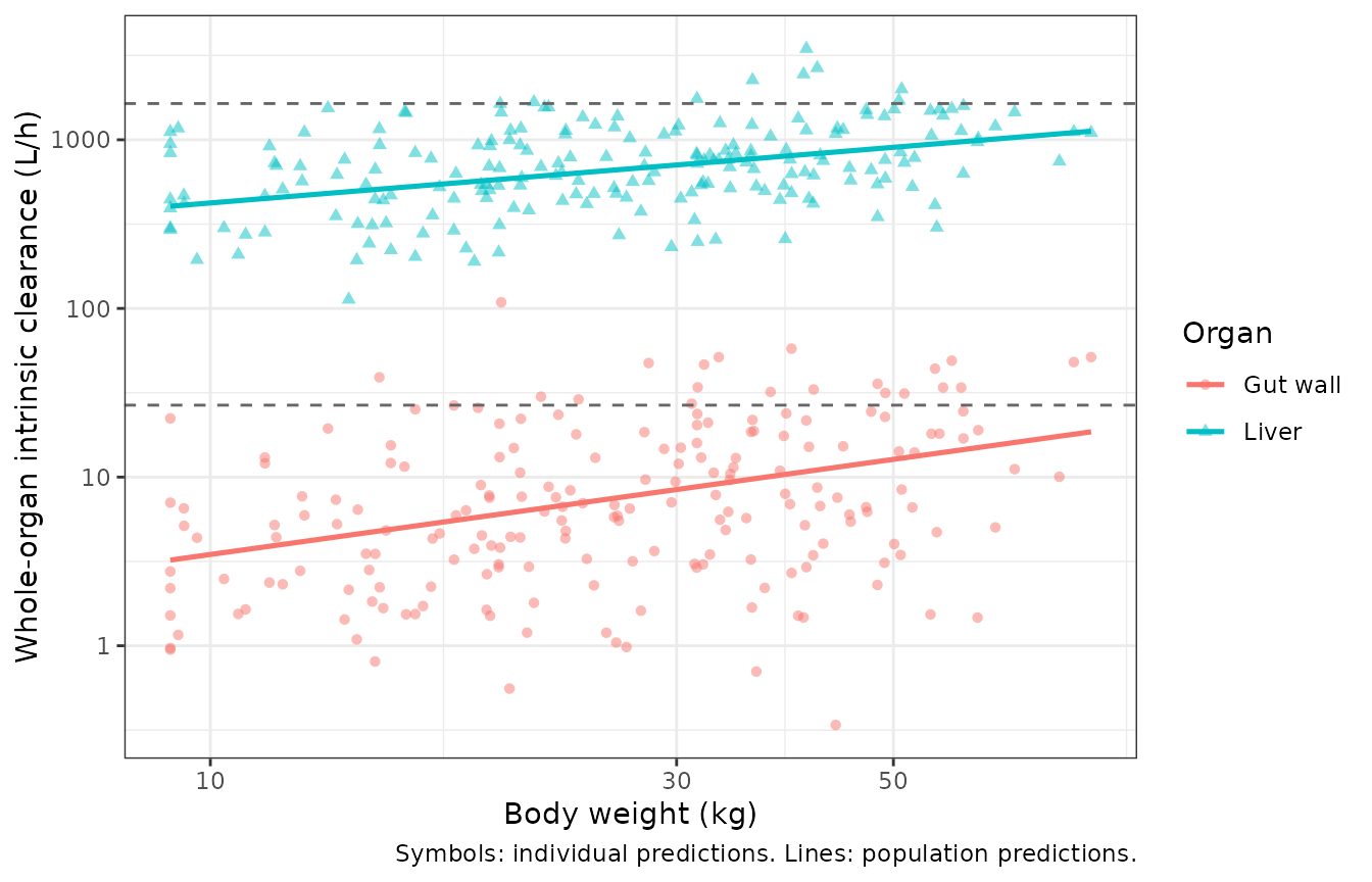
Replicates Figure 2a of Brussee 2018: whole-organ intrinsic clearance versus body weight. Symbols are individual predictions, lines population predictions; dashed lines are the adult literature values.
Figure 2b – intrinsic clearance per gram of organ versus age
Organ weight is the organ volume multiplied by the organ density of 1040 g/L. Adult reference values assume an organ volume of 1 L, i.e. 1040 g of organ.
ORGAN_DENSITY <- 1040 # g/L, Brussee 2018 Model Development

per_g <- function(df) {
  df |>
    dplyr::transmute(
      AGE,
      `Gut wall` = cl_int_g / (v_gut * ORGAN_DENSITY),
      Liver = cl_int_h / (v_liv * ORGAN_DENSITY)
    ) |>
    tidyr::pivot_longer(-AGE, names_to = "Organ", values_to = "clint_per_g")
}

ggplot2::ggplot(per_g(per_subject), ggplot2::aes(AGE, clint_per_g, colour = Organ, shape = Organ)) +
  ggplot2::geom_point(alpha = 0.5) +
  ggplot2::geom_smooth(
    data = per_g(typical_subject),
    method = "loess", formula = y ~ x, se = FALSE
  ) +
  ggplot2::geom_hline(yintercept = 26.7 / ORGAN_DENSITY, linetype = "dashed", colour = "grey40") +
  ggplot2::geom_hline(yintercept = 1640 / ORGAN_DENSITY, linetype = "dashed", colour = "grey40") +
  ggplot2::scale_y_log10() +
  ggplot2::labs(
    x = "Age (years)",
    y = "Intrinsic clearance per gram of organ (L/h/g)",
    caption = "Symbols: individual predictions. Lines: loess of population predictions."
  ) +
  ggplot2::theme_bw()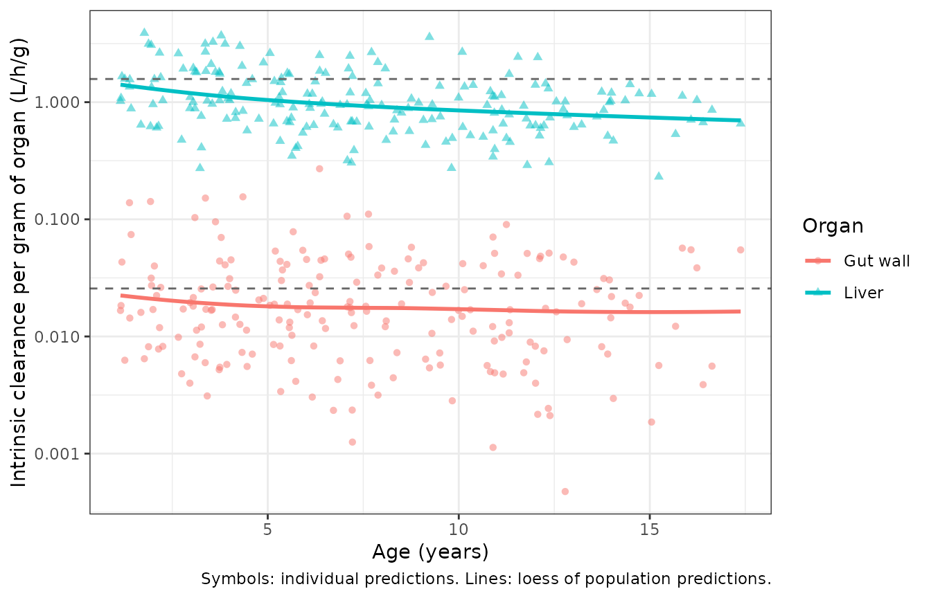
Replicates Figure 2b of Brussee 2018: intrinsic clearance per gram of organ versus age. Dashed lines are the adult reference values.
The paper’s reading of this figure is that hepatic intrinsic CYP3A activity per gram of liver decreases with age, while gut wall activity per gram of small intestine shows “no trend with increasing age … in children >2 year of age” apart from “a small drop around the age of 4-5 years”. Both readings are reproduced: the liver trend is strongly negative, and the gut wall trend is essentially flat once the 1-2 year band is excluded, as the paper qualifies.
# The published trend lines are loess fits of the POPULATION predictions, so
# the rank correlations below are computed on those rather than on the
# individual predictions, whose large CL_G,int IIV (omega^2 = 1.20) would
# swamp any covariate trend.
trend <- typical_subject |>
  dplyr::transmute(
    AGE,
    gut_per_g = cl_int_g / (v_gut * ORGAN_DENSITY),
    liv_per_g = cl_int_h / (v_liv * ORGAN_DENSITY)
  )
rho_liver <- cor(trend$AGE, trend$liv_per_g, method = "spearman")
rho_gut <- cor(trend$AGE, trend$gut_per_g, method = "spearman")
rho_gut_over2 <- with(
  dplyr::filter(trend, AGE > 2),
  cor(AGE, gut_per_g, method = "spearman")
)
cat(sprintf(
  "Spearman rho vs age: liver %.2f | gut wall %.2f (all ages), %.2f (age > 2 y)\n",
  rho_liver, rho_gut, rho_gut_over2
))
#> Spearman rho vs age: liver -0.97 | gut wall -0.37 (all ages), -0.28 (age > 2 y)

# Direction / flatness of the published trends, asserted on whole-cohort rank
# correlations rather than on any individual subject. The cohort covariates come
# from base R's RNG under a fixed seed and do not depend on the rxode2 version.
stopifnot(rho_liver < -0.5, abs(rho_gut_over2) < 0.45)
Figure 3 – total plasma clearance versus body weight
The adult comparison curve of Figure 3 uses the reported adult
whole-organ intrinsic hepatic clearance of 1640 L/h,
Qh = 3.75 * WT^0.75, a fraction unbound of 0.0303 and a
blood:plasma ratio of 0.66, all substituted into eq. 15.
adult_curve <- tibble::tibble(WT = seq(40, 140, length.out = 60)) |>
  dplyr::mutate(
    q_h = 3.75 * WT^0.75,
    cl_plasma = q_h * 1640 * 0.0303 / (q_h + 0.0303 * 1640 / 0.66)
  )

ggplot2::ggplot(per_subject, ggplot2::aes(WT, cl_plasma)) +
  ggplot2::geom_point(alpha = 0.5) +
  ggplot2::geom_line(
    data = dplyr::arrange(typical_subject, WT), ggplot2::aes(WT, cl_plasma),
    colour = "steelblue", linewidth = 0.9
  ) +
  ggplot2::geom_line(
    data = adult_curve, ggplot2::aes(WT, cl_plasma),
    linetype = "dashed", colour = "grey40"
  ) +
  ggplot2::labs(
    x = "Body weight (kg)",
    y = "Total plasma clearance (L/h)"
  ) +
  ggplot2::theme_bw()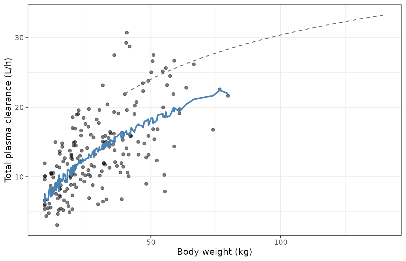
Replicates Figure 3 of Brussee 2018: total plasma clearance versus body weight, with the adult reference curve.
cl_band <- per_subject |>
  dplyr::group_by(ageband) |>
  dplyr::summarise(
    n = dplyr::n(),
    `Median CL (L/h)` = median(cl_plasma),
    .groups = "drop"
  )
knitr::kable(cl_band, digits = 1,
caption = "Median total plasma clearance by age band. Brussee 2018 Figure 3 spans 6.0 L/h in 1-2 year olds to 17.5 L/h in children 16 years and older.")| ageband | n | Median CL (L/h) |
|---|---|---|
| 1-2 y | 25 | 6.8 |
| 3-5 y | 56 | 10.5 |
| 6-11 y | 83 | 14.3 |
| 12-18 y | 36 | 19.2 |
Figure 4 – gut wall, hepatic and total bioavailability by age band
bioav <- per_subject |>
  dplyr::select(ageband, `F gut wall` = fg, `F hepatic` = fh, `F total` = ftotal) |>
  tidyr::pivot_longer(-ageband, names_to = "Term", values_to = "value")

ggplot2::ggplot(bioav, ggplot2::aes(ageband, value, fill = ageband)) +
  ggplot2::geom_boxplot(show.legend = FALSE) +
  ggplot2::facet_wrap(~Term) +
  ggplot2::labs(x = "Age category", y = "Bioavailability (fraction)") +
  ggplot2::theme_bw()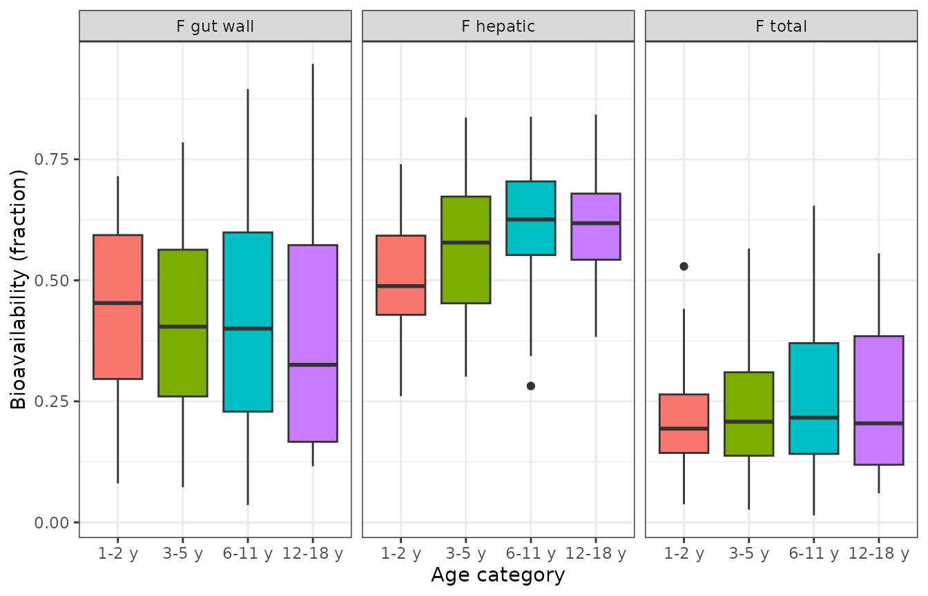
Replicates Figure 4 of Brussee 2018: bioavailability in the gut wall, the liver, and overall, by age category.
band_medians <- function(df, suffix) {
  df |>
    dplyr::group_by(ageband) |>
    dplyr::summarise(
      n = dplyr::n(),
      Fg = median(fg), Fh = median(fh), Ftotal = median(ftotal),
      .groups = "drop"
    ) |>
    dplyr::rename_with(~paste0(.x, suffix), c(Fg, Fh, Ftotal))
}

fig4 <- band_medians(per_subject, " (indiv)") |>
  dplyr::left_join(
    dplyr::select(band_medians(typical_subject, " (pop)"), -n),
    by = "ageband"
  ) |>
  dplyr::mutate(
    `Fg published` = c(0.37, 0.39, 0.34, 0.29),
    `Fh published` = c(0.58, NA, NA, 0.73)
  )

knitr::kable(fig4, digits = 3,
caption = "Median bioavailability terms by age band: individual predictions, population predictions, and the values Brussee 2018 reports (Fh is reported only for the outer two bands).")| ageband | n | Fg (indiv) | Fh (indiv) | Ftotal (indiv) | Fg (pop) | Fh (pop) | Ftotal (pop) | Fg published | Fh published |
|---|---|---|---|---|---|---|---|---|---|
| 1-2 y | 25 | 0.453 | 0.488 | 0.194 | 0.374 | 0.502 | 0.183 | 0.37 | 0.58 |
| 3-5 y | 56 | 0.404 | 0.578 | 0.208 | 0.386 | 0.589 | 0.223 | 0.39 | NA |
| 6-11 y | 83 | 0.400 | 0.626 | 0.216 | 0.374 | 0.627 | 0.233 | 0.34 | NA |
| 12-18 y | 36 | 0.326 | 0.618 | 0.205 | 0.336 | 0.632 | 0.216 | 0.29 | 0.73 |
Concentration-time profiles
prof <- sim |>
  dplyr::filter(!is.na(Cc)) |>
  dplyr::select(id, time, Midazolam = Cc, `1-OH-midazolam` = Cc_1ohm) |>
  tidyr::pivot_longer(c(Midazolam, `1-OH-midazolam`),
                      names_to = "Analyte", values_to = "conc") |>
  dplyr::group_by(Analyte, time) |>
  dplyr::summarise(
    lo = quantile(conc, 0.05), md = median(conc), hi = quantile(conc, 0.95),
    .groups = "drop"
  )

ggplot2::ggplot(prof, ggplot2::aes(time, md, colour = Analyte, fill = Analyte)) +
  ggplot2::geom_ribbon(ggplot2::aes(ymin = lo, ymax = hi), alpha = 0.2, colour = NA) +
  ggplot2::geom_line() +
  ggplot2::coord_cartesian(xlim = c(0, 12)) +
  ggplot2::labs(x = "Time after dose (h)", y = "Whole-blood concentration (nmol/L)") +
  ggplot2::theme_bw()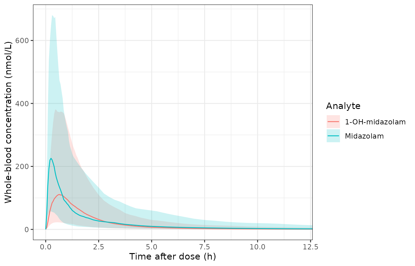
Simulated whole-blood midazolam and 1-OH-midazolam concentrations after a single 10 mg oral dose; median and 5th-95th percentile band across 200 virtual children.
PKNCA validation
Brussee 2018 reports no non-compartmental analysis of its own, so the NCA below characterises the packaged model rather than reproducing a published table. It is run separately for each of the two outputs, grouped by age band so that the maturational trend is visible.
nca_for <- function(sim, conc_col) {
  conc_df <- sim |>
    dplyr::filter(!is.na(.data[[conc_col]])) |>
    dplyr::transmute(id, ageband, time, Cc = .data[[conc_col]])

  dose_df <- conc_df |>
    dplyr::distinct(id, ageband) |>
    dplyr::mutate(time = 0, dose = dose_nmol)

  o_conc <- PKNCA::PKNCAconc(
    conc_df, Cc ~ time | ageband + id,
    concu = "nmol/L", timeu = "h"
  )
  o_dose <- PKNCA::PKNCAdose(
    dose_df, dose ~ time | ageband + id,
    doseu = "nmol"
  )
  PKNCA::pk.nca(PKNCA::PKNCAdata(o_conc, o_dose))
}

nca_parent <- nca_for(sim, "Cc")
nca_metab <- nca_for(sim, "Cc_1ohm")

summarise_nca <- function(res, analyte) {
  res$result |>
    dplyr::filter(PPTESTCD %in% c("cmax", "tmax", "aucinf.obs", "half.life")) |>
    dplyr::group_by(ageband, PPTESTCD) |>
    dplyr::summarise(value = median(PPORRES), .groups = "drop") |>
    tidyr::pivot_wider(names_from = PPTESTCD, values_from = value) |>
    dplyr::mutate(Analyte = analyte, .before = 1)
}

nca_tab <- dplyr::bind_rows(
  summarise_nca(nca_parent, "Midazolam"),
  summarise_nca(nca_metab, "1-OH-midazolam")
) |>
  dplyr::rename(
    `Age band` = ageband,
    `Cmax (nmol/L)` = cmax,
    `Tmax (h)` = tmax,
    `AUC0-inf obs (nmol*h/L)` = aucinf.obs,
    `t1/2 (h)` = half.life
  )

knitr::kable(nca_tab, digits = 2,
caption = "Median simulated NCA parameters by analyte and age band, after a single 10 mg oral midazolam dose.")| Analyte | Age band | AUC0-inf obs (nmol*h/L) | Cmax (nmol/L) | t1/2 (h) | Tmax (h) |
|---|---|---|---|---|---|
| Midazolam | 1-2 y | 428.26 | 332.51 | 2.63 | 0.20 |
| Midazolam | 3-5 y | 375.79 | 301.06 | 3.41 | 0.25 |
| Midazolam | 6-11 y | 292.68 | 207.83 | 5.22 | 0.25 |
| Midazolam | 12-18 y | 199.40 | 127.87 | 7.23 | 0.30 |
| 1-OH-midazolam | 1-2 y | 495.66 | 254.75 | 2.63 | 0.55 |
| 1-OH-midazolam | 3-5 y | 337.10 | 171.12 | 3.41 | 0.55 |
| 1-OH-midazolam | 6-11 y | 235.31 | 98.78 | 5.18 | 0.60 |
| 1-OH-midazolam | 12-18 y | 147.01 | 60.24 | 6.58 | 0.65 |
# Exposure must fall with age for a fixed 10 mg dose, because clearance rises
# with body weight. Asserted on the group medians, not on individual subjects.
auc_by_band <- nca_tab |>
  dplyr::filter(Analyte == "Midazolam") |>
  dplyr::arrange(`Age band`)
stopifnot(
  auc_by_band$`AUC0-inf obs (nmol*h/L)`[1] >
    auc_by_band$`AUC0-inf obs (nmol*h/L)`[nrow(auc_by_band)]
)
Comparison against published results
Because the paper reports derived first-pass and clearance quantities rather than NCA parameters, the validation table compares those directly.
comparison <- tibble::tribble(
  ~Quantity, ~Reference, ~Simulated,
  "Median gut wall bioavailability Fg", 0.34, median(per_subject$fg),
  "Median hepatic bioavailability Fh", 0.66, median(per_subject$fh),
  "Median total bioavailability Ftotal", 0.208, median(per_subject$ftotal),
  "Mean total bioavailability Ftotal", 0.227, mean(per_subject$ftotal),
  "SD of total bioavailability Ftotal", 0.124, sd(per_subject$ftotal),
  "CL_H,int / CL_G,int at 16 kg", 105, ref16$cl_int_h / ref16$cl_int_g
) |>
  dplyr::mutate(`% diff` = 100 * (Simulated / Reference - 1))

knitr::kable(comparison, digits = 3,
caption = "Simulated versus published derived quantities (Brussee 2018 Results and Discussion).")| Quantity | Reference | Simulated | % diff |
|---|---|---|---|
| Median gut wall bioavailability Fg | 0.340 | 0.401 | 17.990 |
| Median hepatic bioavailability Fh | 0.660 | 0.601 | -8.880 |
| Median total bioavailability Ftotal | 0.208 | 0.212 | 2.000 |
| Mean total bioavailability Ftotal | 0.227 | 0.245 | 7.733 |
| SD of total bioavailability Ftotal | 0.124 | 0.139 | 12.304 |
| CL_H,int / CL_G,int at 16 kg | 105.000 | 103.740 | -1.200 |
The paper also reports the spread of each first-pass term across its cohort. These are shown for orientation only and are deliberately not asserted: the extremes of a random cohort are not reproducible across rxode2 versions, which draw different eta samples.
ranges <- tibble::tibble(
  Quantity = c("Fg", "Fh", "Ftotal"),
  `Published range` = c("0.02-0.85", "0.35-0.93", "0.015-0.779"),
  `Simulated range` = c(
    sprintf("%.3f-%.3f", min(per_subject$fg), max(per_subject$fg)),
    sprintf("%.3f-%.3f", min(per_subject$fh), max(per_subject$fh)),
    sprintf("%.3f-%.3f", min(per_subject$ftotal), max(per_subject$ftotal))
  )
)
knitr::kable(ranges, caption = "Published versus simulated spread of the first-pass terms (display only, not asserted).")| Quantity | Published range | Simulated range |
|---|---|---|
| Fg | 0.02-0.85 | 0.036-0.947 |
| Fh | 0.35-0.93 | 0.261-0.842 |
| Ftotal | 0.015-0.779 | 0.014-0.654 |
# Centre-of-distribution checks. Ftotal is the paper's headline result and the
# product of the two first-pass terms, so it gets the tighter bound; Fg and Fh
# individually are each within about 10%.
stopifnot(
  abs(median(per_subject$ftotal) / 0.208 - 1) < 0.15,
  abs(median(per_subject$fg) / 0.34 - 1) < 0.20,
  abs(median(per_subject$fh) / 0.66 - 1) < 0.20
)
The population predictions reproduce the
non-monotone gut wall pattern the paper describes – Fg
rising from the 1-2 year band to the 3-5 year band, then falling through
adolescence – while Fh rises monotonically with age in both
the population and the individual predictions. The per-band medians of
the individual predictions are noisier and do not
preserve the Fg ordering: the between-subject variance on
CL_G,int is 1.20 on the log scale (over 100% CV), and the
bands here hold 25-83 virtual subjects against the paper’s 264, so
band-level medians of individual values carry considerable sampling
noise. The pooled cohort median, mean, SD and range of
Ftotal all match closely (table above), which is the level
at which this cohort is informative.
Assumptions and deviations
Assumptions made in this vignette (not in the paper).
-
Weight-for-age anchor. Individual-level covariates are not
public. The virtual cohort draws weight log-normally (25% spread) around
6.5 + 2.1 * AGE^1.15kg, a median weight-for-age curve that tracks the CDC 50th percentile across 1-18 years (9 kg at 1 year, 26 kg at 7, 43 kg at 12, 61 kg at 17), floored at the study’s minimum observed weight of 9.1 kg. The cohort’s median age and weight then approach the Table SI values of 7 years and 27.4 kg. This anchor is load-bearing for Figure 2b: the per-gram-of-organ trends depend on how fast intrinsic clearance (a power function of weight) grows relative to organ volume (a function of age and body surface area), so a weight-for-age curve that undershoots older children manufactures a spurious downward gut wall trend. The paper’s extreme upper weight (137.6 kg) is an individual outlier that a 200-subject draw from this distribution does not reproduce; every assertion in this vignette is therefore placed on medians, group summaries, rank correlations or exact deterministic quantities, never on a cohort extreme. - Molecular weight. The model is molar, and the paper’s doses are in milligrams. Converting 10 mg to nmol uses the midazolam free-base molecular weight of 325.77 g/mol, which the paper does not print. This scales all simulated concentrations linearly and affects no bioavailability, clearance or extraction-ratio result.
- Age at the hematocrit band edges. Table I’s hematocrit bands are printed as 1-2 y, 3-6 y, 7-12 y and 12-18 y, so the 7-12 and 12-18 bands overlap at exactly 12 years. Age 12 is assigned to the older, sex-split band.
Deviations and source inconsistencies.
-
Fraction unbound: equations versus Figure S2A. Eq. 2
combined with eq. 3 and the Table I constants (
fu_adult0.0303,fu_M,adult0.106,[P]_adult37.7 g/L) yields midazolam plasma protein binding of 96.6-96.9% and 1-OH-midazolam binding of about 88.5-89.2% across the studied age range. The paper’s own text states 96.1-96.4% for midazolam, and Figure S2A of the supplement plots roughly 96.2-96.4% for midazolam and roughly 82.4-83.2% for 1-OH-midazolam. No single alternative value of[P]_adultreconciles the figure for both analytes simultaneously, so the discrepancy cannot be repaired by a unit or constant substitution. The printed equations are used here, per the standing convention that a printed equation outranks prose. This choice is corroborated by the results: it reproduces the paper’s reported medianFh,Ftotaland the Figure 3 clearance range more closely than the figure-implied unbound fractions would, which give a lowerFhthan the paper reports. -
Absorption and time to peak. The paper fixes
kaat 4.16 1/h and states that this yields peak concentrations “round 30 min”. The packaged model peaks at roughly 15 minutes for a typical 27 kg child. This is not an encoding choice that can be adjusted: with the Table II central volume (20.4 L at 76 kg, so 7.4 L at 27.4 kg) and the well-stirred blood clearance implied byCL_H,int(about 21 L/h), the central-compartment rate constant is about 2.9 1/h, and a first-order absorption model cannot place Tmax later than1/kel, i.e. about 21 minutes, for any value ofka. The stated 30 min is therefore not reproducible from the paper’s own Table II values. The distinction matters only for the shape of the early absorption phase;kais a fixed parameter and does not affect the extraction ratios, bioavailability or clearance, which are what the paper reports. -
Hepatic bioavailability offset. The simulated cohort median
Fhis about 0.61 against the reported 0.66, and the medianFgabout 0.35 against the reported 0.34. The two offsets act in opposite directions, so the headlineFtotalmatches closely (0.20 simulated versus 0.208 reported, with mean and SD also close). Part of the residual difference is attributable to the virtual cohort’s covariate distribution differing from the real one. -
Intestinal surface area units. Table I labels the
intestinal surface area column “dm2”, but eqs. 12-14 with radius and
length in metres produce m^2, and the 0.66 m^2 adult cut-off confirms
that scale. The area is treated as m^2 and converted to dm^2 inside the
permeability clearance so that
CL_permcomes out in L/h. Figure S2B of the supplement, which plots intestinal surface area in m^2 and plateaus at 0.66, corroborates this reading. - Height polynomial validity. The supplemental height polynomials (eqs. S1, S2) are Simcyp fits over the paediatric range. They are used unmodified, but are only meaningful for ages 1-18 years; the model should not be extrapolated outside that range.
- No IIV on distribution volumes. The paper could not estimate volumes or their between-subject variability from oral-only data, so all between-subject variability sits on the intrinsic and inter-compartmental clearances. The authors note that these variance terms, and the residual error, may therefore be inflated.
-
Metabolite gut wall clearance.
CL_G,int,Mcould not be estimated independently (“due to model instability”) and is carried as the ratioratio_cl_int_g_1ohm(18.4) times the individual parent gut wall intrinsic clearance, so it inherits the parent’s between-subject variability and its body-weight exponent. That parameter is deliberately not namedlclrat_1ohm: the registeredlclrat_<metab>canonical is the ratio of one elimination route to the parent’s unchanged-elimination clearance for parallel losses from a single compartment, which is a different quantity. -
Dosing route. Only oral dosing was studied. The
centralcompartment is a named ODE state, so intravenous administration can be simulated by dosing it directly – bypassing the gut wall and hepatic first pass – but no IV data informed this model.