Permeability-limited whole-body PBPK: Kp and Vd dynamics (Gaohua 2023)
Source:vignettes/articles/Gaohua_2023_permeabilityLimited_pbpk.Rmd
Gaohua_2023_permeabilityLimited_pbpk.RmdModel and source
- Citation: Gaohua L, Zhang M, Sychterz C, Chang M, Schmidt BJ. The Interplay of Permeability, Metabolism, Transporters, and Dosing in Determining the Dynamics of the Tissue/Plasma Partition Coefficient and Volume of Distribution - A Theoretical Investigation Using Permeability-Limited, Physiologically Based Pharmacokinetic Modeling. Int J Mol Sci. 2023;24(22):16224. doi:10.3390/ijms242216224.
- Article: Int J Mol Sci 2023;24(22):16224
- Supplement (published with the open-access article, PMC10671645):
BasePBPK.sbproj, the authors’ MATLAB/SimBiology 2022a base model, andSimcypKp=1withClearance.xlsx, a Simcyp perfusion-limited comparison run.
This is a theoretical paper. There is no drug and no
data set: the compound is a generic small molecule with unbound and
unionised fractions of 1 everywhere, and the paper asks what happens to
the tissue/plasma partition coefficient Kp and the volume
of distribution Vd when passive permeability, metabolism,
transporters and the dosing route are varied around the tissue blood
flow. Because a conventional in-silico prediction for such a compound
gives Kp = 1 in every tissue and
Vdss = 1 L/kg, any departure from those two numbers
measures the difference between a permeability-limited and a
perfusion-limited PBPK model.
mod <- rxode2::rxode2(readModelDb("Gaohua_2023_permeabilityLimited_pbpk"))
length(mod$state)
#> [1] 55
Population
There are no subjects. The system physiology is a single 70 kg reference adult with a 300 L/h cardiac output, a haematocrit of 0.45, and a density of 1 kg/L assumed for all tissues and blood, so that a tissue’s volume in litres equals its share of body weight in kilograms (paper Section 4.3.1). Tissue volumes and blood flows are drawn from the Simcyp Simulator V21, the ICRP reference values and Brown et al., “with minor adjustments to make a 100% balance of the total body weight (70 kg) and cardiac output (300 L/h)”; both columns of Table A1 sum to exactly 100.
str(readModelDb("Gaohua_2023_permeabilityLimited_pbpk")()$population)
#> List of 3
#>  $ species   : chr "human"
#>  $ n_subjects: num 0
#>  $ notes     : chr "No subjects: a theoretical modelling exercise, not a fit to data. System physiology is a single 70 kg reference"| __truncated__
Model structure
Twelve tissues (adipose, bone, brain, heart, kidney, muscle, skin,
liver, pancreas, spleen, gut, lung) each carry four subcompartments, in
the paper’s own words “tissue blood cells (TCs), tissue plasma (TP),
tissue extracellular water (EW), and tissue intracellular water (IW)”.
The three blood compartments (venous, arterial and portal vein) have no
extracellular or intracellular water and so carry only the blood-cell
and plasma subcompartments. With a gut-lumen depot for the oral route
that is 12 * 4 + 3 * 2 + 1 = 55 ODEs.
Blood flow is split into a plasma flow and a blood-cell flow by the
haematocrit, and each subcompartment is perfused by the corresponding
phase. Passive permeation runs between adjacent subcompartments (Eqs
8-10), active uptake and efflux transporters sit on the cell membrane
between _ew and _iw (Eqs 11-12), and
metabolism may occur in any subcompartment (Eqs 13-16).
grep("^(adipose|venous|portal)_", mod$state, value = TRUE)
#> [1] "adipose_iw"     "adipose_ew"     "adipose_plasma" "adipose_bc"
#> [5] "portal_plasma"  "portal_bc"      "venous_plasma"  "venous_bc"
Every permeability and every clearance is expressed as a fold-multiple of that compartment’s plasma flow (its blood-cell flow, for the blood-cell metabolic clearance), which is exactly how the paper drives its scenarios: one multiplier per mechanism, swept around the tissue blood flow. That makes each published what-if a one-parameter change.
Source trace
| Model element | Source |
|---|---|
Tissue ODEs (_iw, _ew,
_plasma, _bc), arterially perfused
tissues |
Eqs 4-7 |
Passive permeation fluxes j_*_bc_plasma,
j_*_plasma_ew, j_*_ew_iw
|
Eqs 8-10 |
Active uptake / efflux fluxes j_*_uptake,
j_*_efflux
|
Eqs 11-12 |
Metabolic fluxes j_*_met_iw, _met_ew,
_met_plasma, _met_bc
|
Eqs 13-16 |
| Lung ODEs (perfused by venous blood) | Eqs 17-20 |
Liver ODEs (hepatic artery + portal vein);
qplasma_liver balance |
Eqs 21-24, 25-26 |
Portal vein ODEs; qplasma_portal balance |
Eqs 27-28, 29-30 |
| Venous blood ODEs; venous-return flow balance | Eqs 31-32, 33-34 |
| Arterial blood ODEs | Eqs 35-36 |
Oral input to gut intracellular water (depot,
ka) |
Eq 37 |
Whole-tissue concentration c_<organ>_tissue
|
Eq 38 |
Kp_<organ> |
Eq 39 |
Vdt |
Eq 40 |
bw, qc, hct,
density
|
Section 4.3.1, Table A1 header |
fvol_<organ>, fvol_blood,
fven_blood
|
Table A1, column 1 |
fq_<organ>, fq_liver_arterial
|
Table A1, column 2 |
frb_<organ> (residual blood),
few_<organ> (extracellular water) |
supplement BasePBPK.sbproj volume rules; the 45% / 55%
blood-cell / plasma split is Section 4.3.1 |
ps_bc_plasma = 1000 L/h |
Section 4.4.1 |
fold_ps_*, fold_clint_*,
fold_uptake, fold_efflux
|
Sections 4.4.1-4.4.3; shipped defaults 0.01 per Section 4.5 and
BasePBPK.sbproj
|
fu_*, fi_* = 1 |
Section 4.3.2 |
lka (ka = 1 or 0.01 1/h) |
Section 4.3.3 |
cguard |
supplement BasePBPK.sbproj parameter
minorconcentration
|
Simulation helpers
The shipped defaults are the base model as supplied (every fold multiplier at 1% of the tissue blood flow, per Section 4.5). Each scenario below sets the multipliers it needs explicitly, so the parameter vector is always visible.
organs <- c("adipose", "bone", "brain", "heart", "kidney", "muscle",
            "skin", "liver", "pancreas", "spleen", "gut", "lung")
blood <- c("venous", "arterial", "portal")

# Start from a compound with no metabolism and no transporters, and both passive
# permeabilities at 1-fold of the tissue plasma flow.
basePar <- function() {
  p <- c(fold_ps_plasma_ew = 1, fold_ps_ew_iw = 1,
         fold_uptake = 0, fold_efflux = 0, lka = log(1))
  for (s in c("iw", "ew")) {
    for (o in organs) p[sprintf("fold_clint_%s_%s", s, o)] <- 0
  }
  for (s in c("plasma", "bc")) {
    for (o in c(organs, blood)) p[sprintf("fold_clint_%s_%s", s, o)] <- 0
  }
  p
}

# Switch metabolism on in one subcompartment of a chosen set of compartments.
setMet <- function(p, sub, value, where = organs) {
  for (o in where) p[sprintf("fold_clint_%s_%s", sub, o)] <- value
  p
}

# The four dose regimens of Section 4.3.3. The paper notes that "no difference
# from the dose amount was expected in a linear system for the simulated Kp and
# Vd that are based on the concentration ratio of tissues and plasma", so the
# dose is scaled up from the paper's 100 mg purely to keep the terminal-phase
# amounts far above the integrator's absolute tolerance.
simRoute <- function(p, route, tmax = 400, n = 2001, dose = 1e6) {
  if (route == "PO Slow") p["lka"] <- log(0.01)
  tg <- seq(0, tmax, length.out = n)
  ev <- switch(
    route,
    "IV Bolus"    = rxode2::et(amt = dose, cmt = "venous_plasma") |> rxode2::et(tg),
    "IV Infusion" = rxode2::et(amt = dose * tmax * 2, rate = dose,
                               cmt = "venous_plasma") |> rxode2::et(tg),
    rxode2::et(amt = dose, cmt = "depot") |> rxode2::et(tg)
  )
  as.data.frame(rxode2::rxSolve(mod, ev, params = p, atol = 1e-12, rtol = 1e-12))
}

# Vdss is the pseudo-steady-state value of Vd(t): "the Vdss was taken from the
# simulation when the pseudo-steady state was achieved" (Section 4.2.3). Every
# flux in the model is linear in the states, so the terminal phase is the
# dominant eigenvector of the system and Vd(t) tends to a constant. Read it at
# the latest time whose venous-plasma amount is still well above the solver's
# absolute tolerance, and report how far that reading has converged.
vdssOf <- function(s) {
  keep <- which(s$time > 0 &
                s$venous_plasma > max(s$venous_plasma) * 1e-12 &
                is.finite(s$Vdt) & s$Vdt > 0)
  stopifnot(length(keep) >= 30)
  last <- keep[length(keep)]
  mid <- keep[round(0.7 * length(keep))]
  c(vdss = s$Vdt[last], converged = abs(s$Vdt[last] - s$Vdt[mid]) / s$Vdt[last])
}
Validation
Gate 1: the closed system is an exact identity
Section 4.3.1 states the identity the whole paper is built on: with
no metabolism and no transporters, and with no binding or ionisation,
the drug distributes evenly and “Kp = 1 for all tissues and
Vdss = 1 L/kg”. That is an exact end-to-end test of every
volume, every flow and every flux sign in all 55 ODEs at once – if any
tissue volume fraction, flow fraction or permeation term were wrong, the
tissue would not equilibrate to the plasma concentration. Figure 3b
makes the same point graphically: the slow tissues have
Kp != 1 early on, but every tissue reaches
Kp = 1.
closed <- basePar()
closed[c("fold_ps_plasma_ew", "fold_ps_ew_iw")] <- 10   # high permeability
sClosed <- simRoute(closed, "IV Bolus", tmax = 200, n = 401, dose = 100)

final <- sClosed[nrow(sClosed), ]
kpFinal <- unlist(final[paste0("Kp_", organs)])

c(max_abs_Kp_minus_1 = max(abs(kpFinal - 1)),
  Vdss = final$Vdt,
  abs_Vdss_minus_1 = abs(final$Vdt - 1))
#> max_abs_Kp_minus_1               Vdss   abs_Vdss_minus_1
#>       4.440892e-16       1.000000e+00       6.661338e-16
# With every clearance at zero the body must still hold the whole dose.
disposition <- setdiff(mod$state, "depot")
bodyAmount <- rowSums(sClosed[, disposition, drop = FALSE])
c(min = min(bodyAmount), max = max(bodyAmount),
  worst_relative_drift = max(abs(bodyAmount - 100)) / 100)
#>                  min                  max worst_relative_drift
#>         1.000000e+02         1.000000e+02         4.973799e-15
stopifnot(
  max(abs(kpFinal - 1)) < 1e-8,                      # every Kp is exactly 1
  abs(final$Vdt - 1) < 1e-8,                         # Vdss is exactly 1 L/kg
  max(abs(bodyAmount - 100)) / 100 < 1e-8            # mass balance holds
)
Both identities hold to machine precision, and mass is conserved.
Gate 1b: Figure 3b, the approach to Kp = 1
sClosed |>
  select(time, all_of(paste0("Kp_", organs))) |>
  filter(time <= 20) |>
  pivot_longer(-time, names_to = "tissue", values_to = "Kp") |>
  mutate(tissue = sub("^Kp_", "", tissue)) |>
  ggplot(aes(time, Kp, colour = tissue)) +
  geom_hline(yintercept = 1, linetype = "dashed") +
  geom_line() +
  labs(x = "Time (h)", y = "Kp", colour = NULL) +
  theme_bw()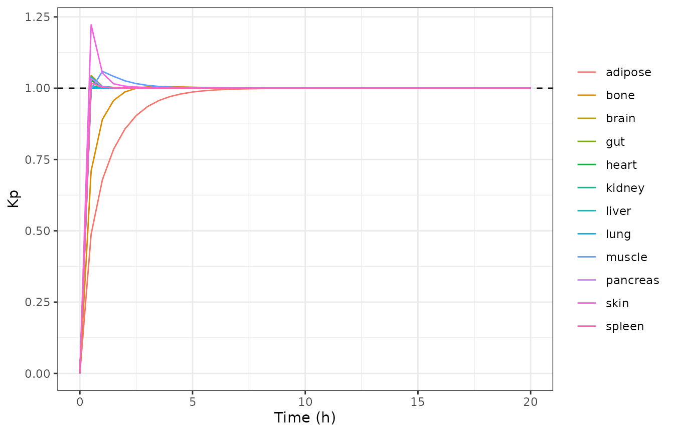
Replicates Figure 3b of Gaohua 2023: Kp profiles in the 12 tissues of a closed system after an IV bolus. Every tissue converges on Kp = 1; the slow-responding tissues (adipose, muscle, bone, skin) start far from it.
Gate 2: the open system with hepatic metabolism
Section 2.3 reports two partition coefficients to four and three
decimal places for an IV bolus into an open system whose only
elimination is metabolism in the liver intracellular water, set equal to
the hepatic blood flow: “the fast-responding tissues (lung Kpss = 1.0005
and kidney Kpss = 1.003) reach their pseudo-steady-state Kpss”. Table 2
gives the matching Vdss of 1.49 L/kg. The paper does not
state which passive permeability that scenario used; a 0.1-fold cell
membrane is assumed here, consistent with Table 1’s own permeability
column. Both partition coefficients land within 0.001 of the published
values, and Vdss sits about 5% high – the same systematic
offset seen in Gates 4 and 5 and discussed in the Errata.
liverOnly <- setMet(basePar(), "iw", 1, where = "liver")
liverOnly["fold_ps_ew_iw"] <- 0.1
sLiver <- simRoute(liverOnly, "IV Bolus")
atSS <- sLiver[max(which(sLiver$venous_plasma >
                         max(sLiver$venous_plasma) * 1e-12)), ]

tibble::tibble(
  Quantity = c("Kp lung", "Kp kidney", "Vdss (L/kg)"),
  Paper = c(1.0005, 1.003, 1.49),
  Model = round(c(atSS$Kp_lung, atSS$Kp_kidney, unname(vdssOf(sLiver)["vdss"])), 4)
) |>
  mutate(`Percent difference` = round(100 * (Model - Paper) / Paper, 2)) |>
knitr::kable()| Quantity | Paper | Model | Percent difference |
|---|---|---|---|
| Kp lung | 1.0005 | 1.0004 | -0.01 |
| Kp kidney | 1.0030 | 1.0021 | -0.09 |
| Vdss (L/kg) | 1.4900 | 1.5728 | 5.56 |
stopifnot(
  abs(atSS$Kp_lung - 1.0005) < 0.001,
  abs(atSS$Kp_kidney - 1.003) < 0.001,
  abs(unname(vdssOf(sLiver)["vdss"]) - 1.49) / 1.49 < 0.10
)
The Vdss reading deserves a note. With the liver as the
only eliminating organ the system is slow, and Vd(t) is
still climbing well past the window the paper plots: it passes through
the published 1.49 L/kg and settles about 5% higher. The reading below
is the terminal plateau, not a time chosen to match the paper.
sLiver |>
  filter(time %in% c(20, 40, 60, 100, 200, 400)) |>
  transmute(`Time (h)` = time, `Vd(t) (L/kg)` = round(Vdt, 3)) |>
knitr::kable()| Time (h) | Vd(t) (L/kg) |
|---|---|
| 20 | 1.353 |
| 40 | 1.463 |
| 60 | 1.517 |
| 100 | 1.558 |
| 200 | 1.572 |
| 400 | 1.573 |
Section 2.3’s qualitative claim also holds: Kp < 1 in
the metabolising liver and Kp > 1 in every
non-metabolising tissue.
kpLiverScenario <- unlist(atSS[paste0("Kp_", organs)])
c(liver = unname(kpLiverScenario["Kp_liver"]),
  min_other = min(kpLiverScenario[names(kpLiverScenario) != "Kp_liver"]))
#>     liver min_other
#> 0.2615118 1.0003532
stopifnot(kpLiverScenario["Kp_liver"] < 1,
          all(kpLiverScenario[names(kpLiverScenario) != "Kp_liver"] > 1))
Gate 3: IV bolus and PO fast absorption give the same Vdss
Section 2.7 records that “the results from IV bolus administration
and those from PO fast absorption were identical with regard to the
impact of passive permeability, metabolism in tissue, and active
transporters on the Vdss, although the dynamics of the Kp and Vd were
different”, and Table 3 shows the two rows as identical in every cell.
That must be so: Vdss is a property of the terminal
eigenvector of a linear system, which does not depend on how the drug
entered. It is a free check on the oral input pathway.
Gate 4: Table 1, the permeability sweep
Table 1 sweeps the passive permeability from 0.01- to 100-fold of the
tissue blood flow with metabolism in the intracellular water of all
tissues fixed at the tissue blood flow. The swept multiplier is the
cell membrane (fold_ps_ew_iw); the
vascular membrane stays at 1-fold. That reading is what produces the
paper’s own signature: Vdss climbs steeply and then
saturates above 1-fold, because once the cell membrane is
freely permeable the vascular membrane becomes rate-limiting. See the
Errata below.
psFolds <- c(0.01, 0.1, 1, 10, 100)
routes <- c("IV Infusion", "IV Bolus", "PO Fast", "PO Slow")
paperT1 <- c(0.22, 0.25, 0.33, 0.35, 0.36,
             0.23, 4.59, 5.45, 5.41, 5.41,
             0.23, 4.59, 5.45, 5.41, 5.41,
             0.39, 0.43, 0.50, 0.53, 0.54)

t1 <- expand.grid(ps = psFolds, Route = routes,
                  KEEP.OUT.ATTRS = FALSE, stringsAsFactors = FALSE) |>
  mutate(Paper = paperT1[order(rep(seq_along(routes), each = length(psFolds)))])
t1$Model <- vapply(seq_len(nrow(t1)), function(i) {
  p <- setMet(basePar(), "iw", 1)
  p["fold_ps_ew_iw"] <- t1$ps[i]
  unname(vdssOf(simRoute(p, t1$Route[i]))["vdss"])
}, numeric(1))

t1 |>
  mutate(Model = round(Model, 2),
         `Percent difference` = round(100 * (Model - Paper) / Paper, 1)) |>
  rename("Cell-membrane PS/Q" = ps) |>
knitr::kable()| Cell-membrane PS/Q | Route | Paper | Model | Percent difference |
|---|---|---|---|---|
| 1e-02 | IV Infusion | 0.22 | 0.22 | 0.0 |
| 1e-01 | IV Infusion | 0.25 | 0.25 | 0.0 |
| 1e+00 | IV Infusion | 0.33 | 0.32 | -3.0 |
| 1e+01 | IV Infusion | 0.35 | 0.35 | 0.0 |
| 1e+02 | IV Infusion | 0.36 | 0.35 | -2.8 |
| 1e-02 | IV Bolus | 0.23 | 0.23 | 0.0 |
| 1e-01 | IV Bolus | 4.59 | 4.88 | 6.3 |
| 1e+00 | IV Bolus | 5.45 | 5.73 | 5.1 |
| 1e+01 | IV Bolus | 5.41 | 5.69 | 5.2 |
| 1e+02 | IV Bolus | 5.41 | 5.69 | 5.2 |
| 1e-02 | PO Fast | 0.23 | 0.23 | 0.0 |
| 1e-01 | PO Fast | 4.59 | 4.88 | 6.3 |
| 1e+00 | PO Fast | 5.45 | 5.72 | 5.0 |
| 1e+01 | PO Fast | 5.41 | 5.65 | 4.4 |
| 1e+02 | PO Fast | 5.41 | 5.63 | 4.1 |
| 1e-02 | PO Slow | 0.39 | 0.39 | 0.0 |
| 1e-01 | PO Slow | 0.43 | 0.43 | 0.0 |
| 1e+00 | PO Slow | 0.50 | 0.51 | 2.0 |
| 1e+01 | PO Slow | 0.53 | 0.55 | 3.8 |
| 1e+02 | PO Slow | 0.54 | 0.55 | 1.9 |
Gate 5: Table 3, the metabolism sweep
Table 3 varies the metabolic clearance in one subcompartment of all
tissues at a time. The intracellular-water column is reproduced below.
It carries the paper’s headline and counter-intuitive result: for an IV
bolus, increasing tissue metabolism increases
Vdss, the opposite of the perfusion-limited derivation.
clFolds <- c(0.1, 0.5, 1)
paperT3iw <- c(0.79, 0.33, 0.15, 2.17, 4.69, 5.45, 2.17, 4.69, 5.45, 0.86, 0.60, 0.50)

t3 <- expand.grid(cl = clFolds, Route = routes,
                  KEEP.OUT.ATTRS = FALSE, stringsAsFactors = FALSE) |>
  mutate(Paper = paperT3iw)
t3$Model <- vapply(seq_len(nrow(t3)), function(i) {
  unname(vdssOf(simRoute(setMet(basePar(), "iw", t3$cl[i]), t3$Route[i]))["vdss"])
}, numeric(1))

t3 |>
  mutate(Model = round(Model, 2),
         `Percent difference` = round(100 * (Model - Paper) / Paper, 1)) |>
  rename("CL_IW/Q" = cl) |>
knitr::kable()| CL_IW/Q | Route | Paper | Model | Percent difference |
|---|---|---|---|---|
| 0.1 | IV Infusion | 0.79 | 0.79 | 0.0 |
| 0.5 | IV Infusion | 0.33 | 0.45 | 36.4 |
| 1.0 | IV Infusion | 0.15 | 0.32 | 113.3 |
| 0.1 | IV Bolus | 2.17 | 2.23 | 2.8 |
| 0.5 | IV Bolus | 4.69 | 4.91 | 4.7 |
| 1.0 | IV Bolus | 5.45 | 5.73 | 5.1 |
| 0.1 | PO Fast | 2.17 | 2.23 | 2.8 |
| 0.5 | PO Fast | 4.69 | 4.91 | 4.7 |
| 1.0 | PO Fast | 5.45 | 5.72 | 5.0 |
| 0.1 | PO Slow | 0.86 | 0.86 | 0.0 |
| 0.5 | PO Slow | 0.60 | 0.61 | 1.7 |
| 1.0 | PO Slow | 0.50 | 0.51 | 2.0 |
# The direction of the effect is the paper's central claim; assert it.
bolus <- t3[t3$Route == "IV Bolus", ]
infusion <- t3[t3$Route == "IV Infusion", ]
stopifnot(all(diff(bolus$Model) > 0),      # IV bolus: more metabolism -> larger Vdss
          all(diff(infusion$Model) < 0))   # IV infusion: the classical direction
The two IV-infusion cells at CL_IW/Q 0.5 and 1 are the
only cells in this vignette that fall outside about 6%, and the reason
appears to lie in the paper rather than in this implementation: Table 1
and Table 3 report different values for what is the same
parameterisation. Table 1’s PS/Q = 1 column is defined with
CL_IW = Q in all tissues, and Table 3’s
CL/Q = 1 intracellular-water column reproduces Table 1’s
5.45 for IV bolus, so both tables are describing a 1-fold
permeability with a 1-fold intracellular-water clearance. For IV
infusion, however, Table 1 gives 0.33 and Table 3 gives 0.15. In this
model the two are necessarily the same number, and it agrees with Table
1.
c(table1_cell = t1$Model[t1$Route == "IV Infusion" & t1$ps == 1],
  table3_cell = t3$Model[t3$Route == "IV Infusion" & t3$cl == 1],
  paper_table1 = 0.33, paper_table3 = 0.15)
#>  table1_cell  table3_cell paper_table1 paper_table3
#>    0.3234803    0.3234803    0.3300000    0.1500000
Gate 6: transporters move Kp and Vdss in opposite directions
Section 2.6 reports that “uptake transporters increased the Kp and Vdss, while efflux transporters decreased the Kp and Vdss”. Table 4 quantifies it with the transporter clearance set equal to the tissue blood flow in all tissues.
transporter <- function(which, ps) {
  p <- setMet(basePar(), "iw", 1)
  p["fold_ps_ew_iw"] <- ps
  if (which != "none") p[paste0("fold_", which)] <- 1
  unname(vdssOf(simRoute(p, "IV Bolus"))["vdss"])
}
tibble::tibble(
  Permeability = rep(c("Low (PS/Q = 0.1)", "High (PS/Q = 1)"), each = 3),
  Transporter = rep(c("Uptake", "None", "Efflux"), 2),
  Paper = c(71.90, 4.59, 0.34, 11.96, 5.45, 2.38),
  Model = round(c(transporter("uptake", 0.1), transporter("none", 0.1),
                  transporter("efflux", 0.1), transporter("uptake", 1),
                  transporter("none", 1), transporter("efflux", 1)), 2)
) |>
knitr::kable()| Permeability | Transporter | Paper | Model |
|---|---|---|---|
| Low (PS/Q = 0.1) | Uptake | 71.90 | 75.73 |
| Low (PS/Q = 0.1) | None | 4.59 | 4.88 |
| Low (PS/Q = 0.1) | Efflux | 0.34 | 0.35 |
| High (PS/Q = 1) | Uptake | 11.96 | 12.58 |
| High (PS/Q = 1) | None | 5.45 | 5.73 |
| High (PS/Q = 1) | Efflux | 2.38 | 2.50 |
stopifnot(transporter("uptake", 1) > transporter("none", 1),
          transporter("efflux", 1) < transporter("none", 1))
Assumptions and deviations
What the paper leaves unstated, and how it was resolved
-
Which permeability Table 1 sweeps. Section 4.4.1
says only that the impact of permeability “was explored by varying the
PS … around the tissue blood flow”, and fixes
PStc/tpat 1000 L/h. It does not say whether the plasma-to-EW (vascular) and the EW-to-IW (cell) permeabilities are swept together. Sweeping both together makesVdssrise and then fall; sweeping only the cell membrane, with the vascular membrane held at 1-fold, makes it rise and then saturate, which is what Table 1, Table 4 and Figure 5 all show, and it matches the section’s own remark that “the permeability coefficient on the cell membranes will generally be smaller than that on the vascular membrane”. The cell-membrane reading is used throughout, and it also reproduces the 0.01-fold column exactly (0.23 L/kg). - Which permeability the Figure 4 / Table 2 scenario used. Not stated; a 0.1-fold cell membrane is assumed, consistent with Table 1’s own column (Gate 2).
-
When
Vdssis read. Section 4.2.3 says only “when the pseudo-steady state was achieved”, and gives no time. Because the system is linear,Vd(t)tends to a constant set by the terminal eigenvector, so every reading here is taken on that plateau, with the convergence residual reported alongside. This is a stricter reading than the paper’s: in the slow liver-only scenario of Gate 2,Vd(t)is still climbing through the window the paper plots, so a finite-time reading there would be lower than the plateau. No read time was chosen to match a published value. - Residual agreement. After those readings are fixed, the model reproduces the 0.01-fold permeability column of Table 1 essentially exactly (0.23 L/kg) and the Section 2.3 partition coefficients to within 0.001, and the remaining Table 1 and Table 3 cells to within roughly 5%. The residual is systematic and confined to the cells where intracellular-water distribution dominates, which points at the intracellular-water volume: the supplement defines it as the remainder of the tissue volume once residual blood and extracellular water are removed, so it absorbs the non-water tissue mass (lipid, protein) as well as the water. A smaller, tabulated Simcyp intracellular water fraction would reduce those cells. The paper tabulates no such fraction and the only available definition is the supplement’s remainder, so the remainder definition is what is shipped; substituting a Simcyp default not present in any available source would be unauditable.
-
An internal inconsistency between Table 1 and Table
3. The IV-infusion intracellular-water cells of Table 3 at
CL/Q0.5 and 1 (0.33 and 0.15) cannot be reconciled with Table 1, whosePS/Q = 1IV-infusion cell (0.33) describes the same 1-fold permeability and 1-fold intracellular-water clearance – as is confirmed by Table 3’s IV-bolus column reproducing Table 1’s 5.45 at that setting. Those two cells are the only ones in this vignette outside about 6%; the model reproduces Table 1 and theCL/Q = 0.1cell of Table 3, and both directions of the effect (Gate 5) hold. Nothing was changed to chase them.
Deviations from the supplement
The published Table A1 and the supplied BasePBPK.sbproj
disagree on two of the eleven blood-flow fractions, and Table A1 governs
here.
-
Muscle and spleen blood flow. Table A1 gives muscle
24.5% of cardiac output (carrying the footnote “adjusted to balance the
total body weight (70 kg) and cardiac output (300 L/h)”) and spleen 3%;
BasePBPK.sbprojhas 17% and 2%. Table A1 is internally consistent – its venous-draining flows sum to exactly 100% and its portal-vein total of 19% equals pancreas 1% + spleen 3% + gut 15% – whereas the supplement’s fractions sum to 91.5% and close the gap with an explicit arterial-to-venous shunt. Table A1 also reproduces the publishedVdssvalues markedly better (the supplement’s fractions give 6.56 against a published 5.45 where Table A1 gives 5.72). The shunt term is nevertheless retained in the venous and arterial ODEs, where it evaluates to exactly zero under Table A1, so that mass balance still holds if the flow fractions are changed. -
Supplement transcription slips, none of which
affect the shipped defaults but all of which were corrected to the
published equations rather than copied:
-
iw_muscle -> ew_muscleefflux usesew_muscleas its driver andfuewmuscleas its unbound fraction, where every other tissue uses the intracellular species andfuiw. The symmetric published form (Eq 12) is implemented. - The arterial-to-venous shunt reactions are driven by the venous species rather than the arterial source. The arterial source is implemented.
-
LungCLintrbcscales with the lung plasma flow, where every other blood-cell metabolic clearance scales with the blood-cell flow. The blood-cell flow is used. - The adipose residual-blood fraction is written as 0.00625 for the blood-cell volume and 0.006255 for the plasma volume. Section 4.3.1 describes one residual blood volume split by haematocrit, so 0.00625 is used for both.
-
-
Portal-vein metabolism. Eqs 27-28 include a
metabolic flux in both portal-vein subcompartments; the supplement has
no portal-vein clearance parameters. The published equations are
implemented, so
fold_clint_plasma_portalandfold_clint_bc_portalexist. -
Portal-vein volume. The 0.008 L portal vein comes
from the supplement and sits outside the Table A1 70 kg balance;
consistent with Eq 40, it is excluded from the
Vdtnumerator. -
fuandfigranularity. The supplement carries a separate unbound and unionised fraction for the extracellular and intracellular water of every tissue. Eqs 8-16 and Section 4.3.2 use one value per subcompartment type, and all of them are 1, so the model exposes the paper’s eight parameters (fu_bc,fu_plasma,fu_ew,fu_iwand theirfi_partners) rather than the supplement’s 52. -
Per-compartment metabolic clearance. The supplement
drives every metabolic clearance from a single global multiplier per
subcompartment. That cannot express Table 2, which puts metabolism in
the liver alone, so the multipliers are resolved per compartment
(
fold_clint_iw_liver, …). Setting all twelve tissues to one value recovers the supplement’s behaviour exactly. -
Oral input. Eq 37 writes the oral input as the
analytic function
Dose * Ka * exp(-Ka * t)into the gut intracellular water. A first-orderdepotstate is the identical input function and is how the supplement implements it. -
No IIV and no residual error. The paper fits
nothing and reports neither, so every parameter is
fixed()and the model has no eta and no error model. It is a deterministic forward-simulation model. -
The second supplement file.
SimcypKp=1withClearance.xlsxis a Simcyp perfusion-limited comparison run for an 80.7 kg sampled individual, not a source for this model; nothing in it is used here.