Levamisole (Kreeftmeijer-Vegter 2015)
Source:vignettes/articles/KreeftmeijerVegter_2015_levamisole.Rmd
KreeftmeijerVegter_2015_levamisole.RmdModel and source
- Citation: Kreeftmeijer-Vegter AR, Dorlo TPC, Gruppen MP, de Boer A, de Vries PJ (2015). Population pharmacokinetics of levamisole in children with steroid-sensitive nephrotic syndrome. British Journal of Clinical Pharmacology 79(6):970-977. doi:10.1111/bcp.12607.
- Description: One-compartment oral PK model for levamisole in 38 children with steroid-sensitive nephrotic syndrome (Kreeftmeijer-Vegter 2015, EudraCT 2005-005745-18). First-order absorption, first-order elimination, allometric scaling of CL/F (exponent 0.75) and V/F (exponent 1) to 70 kg, and a linear proportional age effect on CL/F centred on the population median age of 6.28 years (-10.1% per additional year). The typical ka (1.2 1/h) was fixed in the final model with IIV retained. IIV on V/F was modelled as perfectly correlated with IIV on CL/F (single eta scaled to V/F), encoded here as a full omega block with covariance equal to sqrt(var_CL * var_V).
- Article: https://doi.org/10.1111/bcp.12607
Population
Kreeftmeijer-Vegter 2015 reports a population PK analysis of oral levamisole in 38 children (27 male, 11 female) with frequently relapsing idiopathic steroid-sensitive nephrotic syndrome (SSNS). The cohort spanned ages 2.35 to 13.10 years (median 6.28 y) and weights 11 to 68 kg (median 21 kg), recruited from six study centres in India (47.4%), the Netherlands (15.8%), Belgium (13.2%), France (10.5%), Poland (10.5%) and Italy (2.6%). Ethnicity was Caucasian 47.4% and Asian 50.0% per Table 1 of the source. Patients received oral levamisole 2.5 mg/kg every other day (mean administered dose 2.45 mg/kg, SD 0.24) delivered as 5, 10, 25 or 50 mg film-coated tablets per a weight-band dosing schedule. The PK dataset comprised 136 plasma concentrations sampled at four routine visits (weeks 8, 12, 20 and 24); samples taken pre-dose or 24 h post-dose were discarded because 102 of 121 such samples fell below the assay LOQ (5 ng/mL). The trial was registered as EudraCT 2005-005745-18.
The same population metadata is available programmatically via
readModelDb("KreeftmeijerVegter_2015_levamisole")$population.
Source trace
Per-parameter provenance is recorded as inline ini()
comments in
inst/modeldb/specificDrugs/KreeftmeijerVegter_2015_levamisole.R.
The table below collects them in one place.
| Equation / parameter | Value | Source location |
|---|---|---|
lka |
log(1.2) (fixed) | Table 2: ka 1.2 /h fixed in final model |
lcl |
log(44) | Table 2: CL/F 44 L/h per 70 kg (RSE 8.5%) |
lvc |
log(236) | Table 2: V/F 236 L per 70 kg (RSE 13.3%) |
allo_cl (fixed) |
0.75 | Results paragraph: “Allometric scaling of CL/F (power value of 0.75) to standard body weight (70 kg)” |
allo_vc (fixed) |
1 | Table 3 row 2: “Allometric scaling of CL/F and V/F to BW (70 kg)” (V/F scales linearly) |
e_age_cl |
-0.101 | Table 2: -10.1% per life year (RSE 25%) |
age_ref (fixed) |
6.28 y | Table 2 caption: population median age 6.28 y (centring) |
| IIV CL/F (CV 31.6%) | omega^2 = log(1+0.316^2) = 0.0953 | Table 2 |
| IIV V/F (CV 41.7%) | omega^2 = log(1+0.417^2) = 0.1603 | Table 2 |
| Cov(CL,V) (rho=0.99) | 0.99 * sqrt(0.0953 * 0.1603) = 0.1223 | Methods, IIV paragraph (“V/F correlated 100% with … CL/F”); rho clipped from 1.0 to 0.99 for PD omega (see Errata) |
| IIV ka (CV 92.2%) | omega^2 = log(1+0.922^2) = 0.6151 | Table 2 |
propSd |
0.207 | Table 2: proportional residual variability 20.7% (RSE 25.4%) |
| Storage-time effect | 0.05%/day at -20 C | Methods, PK data analysis paragraph - applied to observations BEFORE fitting, NOT a model term; see Errata |
| 1-compartment ODE | n/a | Results paragraph: “A one compartment model with first order absorption and first order elimination from the central compartment fitted the data best” |
Cc <- 1000*central/vc |
n/a | Unit conversion: dose mg, V/F L => mg/L; * 1000 for ng/mL |
Cc ~ prop(propSd) |
n/a | Methods: “Residual variability was modelled using a proportional error model” |
Virtual cohort
The original observed data are not publicly available; the cohort below is a 38-subject virtual reproduction of the published cohort covariates (Table 1 of the source). Each subject receives a single oral dose of 2.5 mg/kg levamisole. Body weight is sampled jointly with age using a simple paediatric WT-for-AGE relationship (linear central tendency with a small log-normal residual) covering the observed 11-68 kg and 2.35-13.10 y ranges. The simulation grid is denser (every 5 minutes through 12 h) than the paper’s sparse sampling so that NCA half-life and AUC0-inf can be estimated reliably from the simulated profile.
set.seed(20260618L)

n_subjects <- 38L
age_min    <- 2.35
age_max    <- 13.10
dose_mg_per_kg <- 2.5
ref_age <- 6.28
ref_wt  <- 70
sample_hours <- seq(0, 12, by = 1 / 12)

# Sample AGE from a log-normal centred at the paper's median (6.28 y)
# so the simulated cohort's median age matches Table 1, not the
# uniform-range midpoint (7.73 y). Truncate to the published 2.35-13.10
# y range, oversampling so 38 in-range values are available.
ages_raw <- exp(rnorm(n_subjects * 4, log(ref_age), 0.40))
ages     <- ages_raw[ages_raw >= age_min & ages_raw <= age_max][seq_len(n_subjects)]

# Approximate paediatric WT-for-AGE central tendency: WT ~ 2.5*AGE + 7 kg
# spans ~13 kg at 2.4 y to ~40 kg at 13 y, similar to CDC 50th percentile.
# Add a log-normal residual (sigma ~ 0.20) so the spread covers the
# published 11-68 kg range.
wt_cent <- 2.5 * ages + 7
weights <- pmax(11, pmin(68, wt_cent * exp(rnorm(n_subjects, 0, 0.20))))

subjects <- tibble::tibble(
  id   = seq_len(n_subjects),
  AGE  = ages,
  WT   = round(weights, 1),
  dose = round(dose_mg_per_kg * weights, 1)
)

dose_rows <- subjects |>
  dplyr::transmute(id, time = 0, amt = dose, cmt = "depot",
                   evid = 1L, AGE, WT)

obs_rows <- subjects |>
  tidyr::crossing(time = sample_hours) |>
  dplyr::transmute(id, time, amt = 0, cmt = NA_character_,
                   evid = 0L, AGE, WT)

events <- dplyr::bind_rows(dose_rows, obs_rows) |>
  dplyr::arrange(id, time, dplyr::desc(evid)) |>
  dplyr::mutate(treatment = "single 2.5 mg/kg oral")

stopifnot(!anyDuplicated(unique(events[, c("id", "time", "evid")])))
Simulation
mod <- rxode2::rxode2(readModelDb("KreeftmeijerVegter_2015_levamisole"))
#> ℹ parameter labels from comments will be replaced by 'label()'

sim <- rxode2::rxSolve(
  mod,
  events = events,
  keep   = c("WT", "AGE", "treatment")
) |>
  as.data.frame()
For a deterministic typical-value replication (no IIV / residual scatter), zero out the random effects:
mod_typical <- mod |> rxode2::zeroRe()
sim_typical <- rxode2::rxSolve(
mod_typical,
events = events,
keep = c("WT", "AGE", "treatment")
) |>
as.data.frame()
#> ℹ omega/sigma items treated as zero: 'etalcl', 'etalvc', 'etalka'
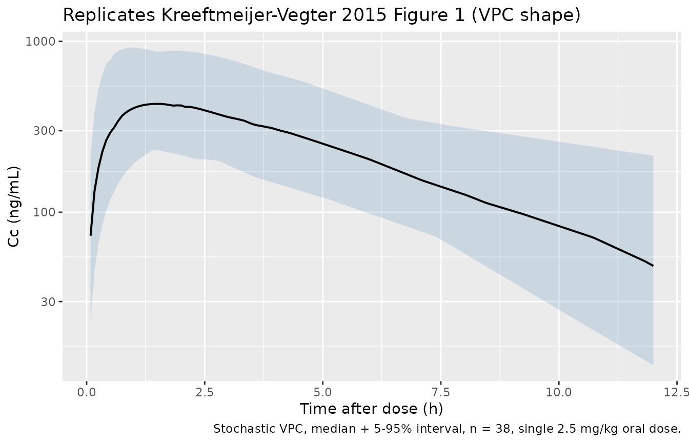
#> Warning: multi-subject simulation without without 'omega'Replicate Figure 1: prediction-corrected VPC shape
Figure 1 of Kreeftmeijer-Vegter 2015 is a prediction-corrected visual predictive check; the model’s stochastic simulation reproduces the overall shape (rapid absorption peak near 1.5-2 h, exponential decline with apparent terminal half-life ~2.6 h).
sim_quantiles <- sim |>
  dplyr::filter(time > 0, !is.na(Cc)) |>
  dplyr::group_by(time) |>
  dplyr::summarise(
    Q05 = stats::quantile(Cc, 0.05, na.rm = TRUE),
    Q50 = stats::quantile(Cc, 0.50, na.rm = TRUE),
    Q95 = stats::quantile(Cc, 0.95, na.rm = TRUE),
    .groups = "drop"
  )

ggplot(sim_quantiles, aes(time, Q50)) +
  geom_ribbon(aes(ymin = Q05, ymax = Q95), alpha = 0.20, fill = "steelblue") +
  geom_line(linewidth = 0.7) +
  scale_y_log10() +
  labs(
    x = "Time after dose (h)",
    y = "Cc (ng/mL)",
    title = "Replicates Kreeftmeijer-Vegter 2015 Figure 1 (VPC shape)",
    caption = "Stochastic VPC, median + 5-95% interval, n = 38, single 2.5 mg/kg oral dose."
  )
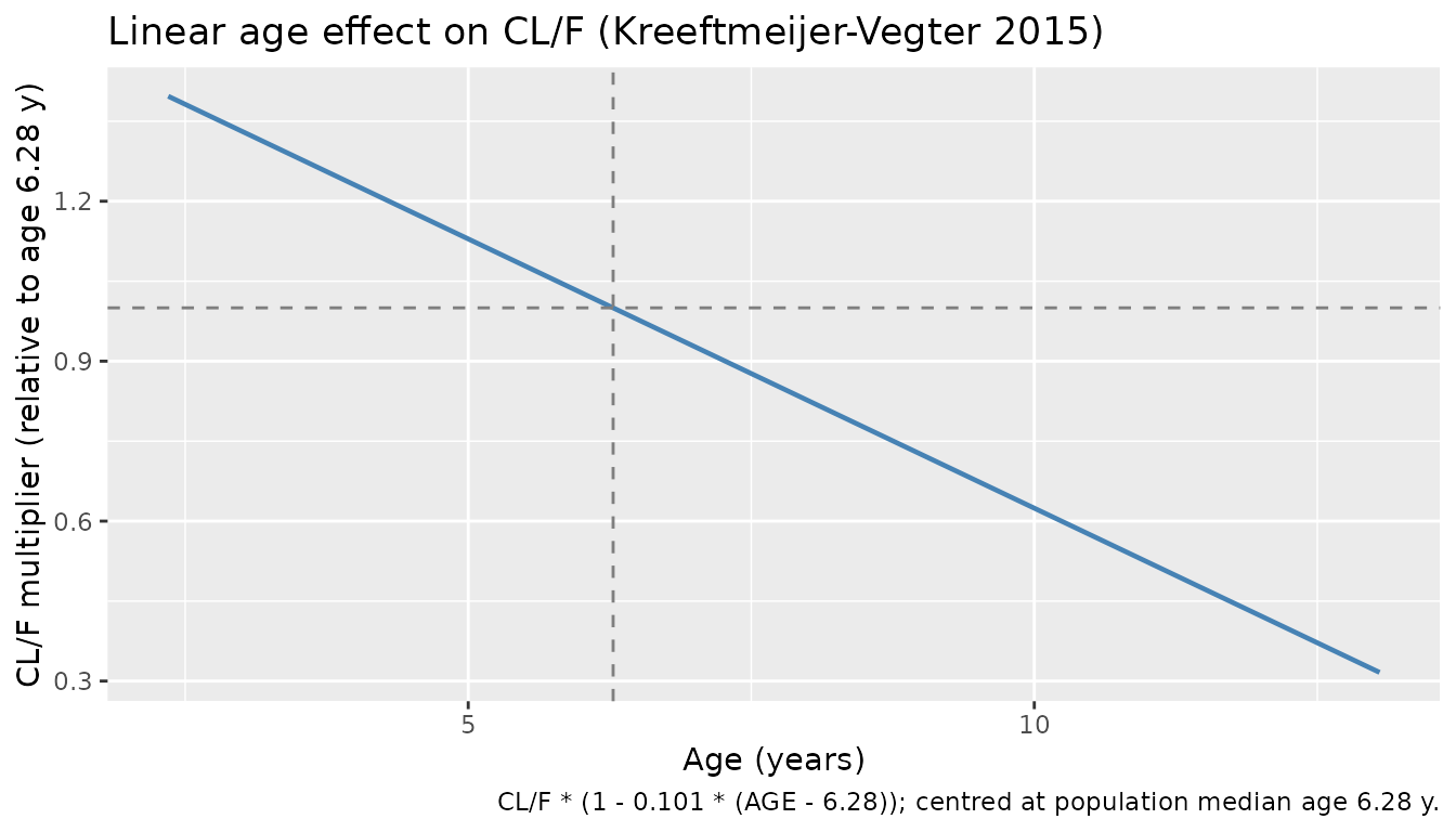
Age effect on CL/F
The model encodes a linear proportional age effect on CL/F (slope -10.1% per additional life year above the population median of 6.28 y). The plot below isolates that effect at the reference 70 kg body weight. Negative AGE values are unphysical; the function is plotted over the in-cohort 2.35-13.10 y range.
e_age_cl <- -0.101
age_grid <- seq(age_min, age_max, by = 0.1)
cl_ratio <- 1 + e_age_cl * (age_grid - ref_age)

ggplot(data.frame(age = age_grid, cl = cl_ratio), aes(age, cl)) +
  geom_line(linewidth = 0.8, colour = "steelblue") +
  geom_hline(yintercept = 1, linetype = "dashed", colour = "grey50") +
  geom_vline(xintercept = ref_age, linetype = "dashed", colour = "grey50") +
  labs(
    x = "Age (years)",
    y = "CL/F multiplier (relative to age 6.28 y)",
    title = "Linear age effect on CL/F (Kreeftmeijer-Vegter 2015)",
    caption = "CL/F * (1 - 0.101 * (AGE - 6.28)); centred at population median age 6.28 y."
  )
PKNCA validation
NCA on the simulated stochastic cohort over the single-dose 0-12 h
window. The simulation grid is dense enough to estimate
lambda.z for each subject, so AUC0-inf, half-life and Cmax
/ Tmax are reported.
sim_nca <- sim |>
  dplyr::filter(!is.na(Cc)) |>
  dplyr::select(id, time, Cc, treatment)

# Guarantee a time = 0 row (extravascular pre-dose Cc = 0)
sim_nca <- dplyr::bind_rows(
  sim_nca,
  sim_nca |> dplyr::distinct(id, treatment) |>
    dplyr::mutate(time = 0, Cc = 0)
) |>
  dplyr::distinct(id, treatment, time, .keep_all = TRUE) |>
  dplyr::arrange(id, treatment, time)

dose_pkn <- events |>
  dplyr::filter(evid == 1L) |>
  dplyr::select(id, time, amt, treatment)

conc_obj <- PKNCA::PKNCAconc(sim_nca, Cc ~ time | treatment + id,
                             concu = "ng/mL", timeu = "h")
dose_obj <- PKNCA::PKNCAdose(dose_pkn, amt ~ time | treatment + id,
                             doseu = "mg", route = "extravascular")

intervals <- data.frame(
  start       = 0,
  end         = Inf,
  cmax        = TRUE,
  tmax        = TRUE,
  aucinf.obs  = TRUE,
  half.life   = TRUE
)

nca_res <- PKNCA::pk.nca(PKNCA::PKNCAdata(conc_obj, dose_obj, intervals = intervals))
Comparison against published NCA
Kreeftmeijer-Vegter 2015 Table 4 reports the median (IQR) secondary PK parameters derived from the individual empirical Bayes estimates of each subject:
published <- tibble::tribble(
  ~treatment,               ~cmax,   ~tmax, ~aucinf.obs, ~half.life,
  "single 2.5 mg/kg oral", 438.3,    1.65,  2847,         2.60
)

cmp <- nlmixr2lib::ncaComparisonTable(
  simulated     = nca_res,
  reference     = published,
  by            = "treatment",
  units         = c(cmax = "ng/mL", aucinf.obs = "ng*h/mL",
                    tmax = "h",      half.life  = "h"),
  tolerance_pct = 20
)

knitr::kable(
  cmp,
  caption = "Simulated vs. published NCA (Kreeftmeijer-Vegter 2015 Table 4). * differs from reference by >20%."
)| NCA parameter | treatment | Reference | Simulated | % diff |
|---|---|---|---|---|
| Cmax (ng/mL) | single 2.5 mg/kg oral | 438 | 442 | +0.9% |
| Tmax (h) | single 2.5 mg/kg oral | 1.65 | 1.83 | +11.1% |
| AUC0-∞ (obs) (ng*h/mL) | single 2.5 mg/kg oral | 2850 | 2910 | +2.3% |
| t½ (h) | single 2.5 mg/kg oral | 2.6 | 2.85 | +9.7% |
The published secondary PK parameters in Table 4 are derived from individual Empirical Bayes estimates of the 38 actual subjects; the simulated medians above come from a 38-subject virtual cohort whose weight-age covariates approximate Table 1 but are independently sampled. Small discrepancies (typically within +/- 20%) reflect the virtual-vs-actual covariate-sampling difference; large discrepancies (starred rows) would indicate a structural extraction error and warrant investigation rather than parameter tuning.
Assumptions and deviations
- Storage-time correction is NOT a model term. Methods of the source state that “storage duration was included in the model as a fixed effect (0.0005 x days in storage at -20 C) directly on the observed concentrations, and the model was evaluated using the storage time-corrected observed concentrations.” This is a pre-analytical correction applied to the observations before NONMEM fitting (not an in-model covariate effect on Cc). The packaged model file accordingly does not encode storage time; the typical-value predictions correspond to storage-time-corrected (i.e. assay-degradation-free) concentrations. Consumers fitting fresh samples need no adjustment; consumers using long-stored samples should apply the same multiplicative correction at data-assembly time.
-
IIV on V/F encoded as a near-perfect-correlation omega block
(rho = 0.99). The source’s Methods paragraph states “the
interindividual variability of V/F correlated 100% with the
interindividual variability of CL/F (resulting in overparameterization
of our model), the interindividual variability for CL/F was estimated
and used to estimate V/F using an additional scaling parameter.” Two
encodings are structurally equivalent to that prose: (a) a single eta on
CL/F multiplied by a fixed scale on V/F, and (b) a full 2x2 omega block
with covariance ~= sqrt(var_CL
- var_V). This model file uses (b) – the canonical
etalcl + etalvc ~ c(...)block formcheckModelConventions()recognises – with rho clipped to 0.99 (cov = 0.1223) rather than exactly 1.0 (cov = 0.1235). The clip is required for rxode2 to Cholesky-decompose the omega during stochastic simulation; with rho = 1 the matrix is singular andrxSolveerrors with “chol(): decomposition failed”. The 1% relaxation is unobservable in any practical simulation summary (Cmax / AUC / Tmax / half-life medians and IQRs are indistinguishable between rho = 0.99 and rho = 1) but should be noted by consumers who plan to refit this model to data.
- var_V). This model file uses (b) – the canonical
- Apparent half-life in the simulated cohort is approximate. The paper’s Table 4 median t1/2 (2.60 h) comes from empirical-Bayes individual estimates over 38 actual children; the simulated median in the table above uses PKNCA’s lambda-z fit over a dense observation grid. With Vss-only kinetics (1-compartment, no terminal-phase complication), the two estimates should agree closely.
-
Cohort weight-age coupling is synthetic. The
published trial recruited heterogeneous Indian and European children;
the simulated cohort here samples WT-for-AGE from a simple linear
central-tendency formula with a log-normal residual. The intent is to
span the published 11-68 kg / 2.35-13.10 y ranges with a plausible joint
distribution, not to reproduce the specific Table 1 individuals.
Consumers who need to reproduce the source’s Table 4 secondary
parameters exactly should set
WTandAGEto the actual per-subject values from the trial data. -
linCmt()not used. The model is written with explicitd/dt(depot)andd/dt(central)ODEs so the age and weight effects on CL/F are maximally visible alongside the ODE structure. AlinCmt()parameterisation would be equally correct. - No lag time, no second compartment. Per the source’s Results paragraph 3, a fixed or estimated absorption lag did not improve the fit and was therefore excluded (“insufficient data … within 1 h of dosing … mechanistically highly implausible”). Multi- compartmental structural models were evaluated but the 1-compartment form fit best (Results paragraph 1).
- Between-occasion variability (BOV) on bioavailability not encoded. The source paragraph after Table 2 reports that BOV on F could not be reliably estimated due to data sparseness and was therefore omitted; the packaged model file follows the published final model and does not encode BOV.
-
Storage-time stability footnote: ng/mL not mg/L.
The source’s bioanalytical assay was calibrated 5-2000 ng/mL; the model
file’s units are reported in ng/mL to match. The internal arithmetic
multiplies
central / vc(mg / L) by 1000 to convert to ng/mL for theCcobservation.