Ivermectin, dengue virus and NS1 (Ding 2024)
Source:vignettes/articles/Ding_2024_ivermectin.Rmd
Ding_2024_ivermectin.RmdModel and source
- Citation: Ding J, Mairiang D, Prayongkul D, Puttikhunt C, Noisakran S, Kaewjiw N, Songjaeng A, Prommool T, Tangthawornchaikul N, Angkasekwinai N, Suputtamongkol Y, Lapphra K, Chokephaibulkit K, White NJ, Avirutnan P, Tarning J. In-host modeling of dengue virus and non-structural protein 1 and the effects of ivermectin in patients with acute dengue fever. CPT Pharmacometrics Syst Pharmacol. 2024;13(12):2196-2208. doi:10.1002/psp4.13233
- Description: In-host dengue virus and non-structural protein 1 (NS1) kinetic model with ivermectin population PK-PD in Thai adults and children with acute dengue fever (Ding 2024). Ivermectin PK: two-compartment disposition with a dose compartment plus six transit absorption compartments (ktr = 7 / MTT), relative bioavailability fixed to 1 with IIV, and allometric body-weight scaling (estimated exponents, centred on 70 kg). Dengue viral load: target-cell-limited model (target cells, an infected-cell eclipse chain of four compartments, virus-producing cells, free virus) with innate clearance c and an antibody-driven neutralisation term kA * A(t) * V, where A(t) is the mean of the normalised sigmoidal-Emax time courses of dengue-specific IgM and IgG. NS1: secreted from producing cells through nine transit compartments with a time-dependent sigmoidal-Emax secretion rate and a first-order elimination rate that rises linearly with time when NS1-specific IgG exceeds a cut-off. Ivermectin inhibits NS1 secretion through an Emax function of its plasma concentration (Emax fixed to 0.99); it has no effect on viral load. Model time is days since infection (fever onset assumed on day 6).
- Article: https://doi.org/10.1002/psp4.13233 (open access; the Supplementary Material holds the ivermectin PK and dengue IgM / IgG parameter tables and the NONMEM code of all four sub-models)
Ding et al. modelled ivermectin pharmacokinetics, dengue viral load
and plasma non-structural protein 1 (NS1) antigen in Thai adults and
children with acute dengue fever. The four sub-models (ivermectin PK,
dengue-specific IgM / IgG time courses, target-cell-limited viral
kinetics, NS1 kinetics) were fitted sequentially, but the authors
simulate them as one coupled system: the antibodies drive viral
neutralisation, the virus-producing cells feed NS1 secretion, and the
ivermectin concentration inhibits NS1 secretion. The package therefore
ships them as one model, Ding_2024_ivermectin.
Model time is days since infection. The authors back-calculated the infection time from the recorded fever onset assuming a 6-day incubation period, so fever onset is day 6 and “dosing on day 7” means 24 h after fever onset. The antibody time courses and the NS1 secretion rate are explicit functions of that time, so event tables must start at the infection (time 0), not at the first dose.
Population
The analysis pooled the ESIDEN phase II/III placebo-controlled trial in adults (NCT02045069; 250 enrolled at Siriraj Hospital, Bangkok and Loei Hospital; ivermectin 400 ug/kg once daily for 2 or 3 days, or placebo) and the PKIDEN paediatric PK-PD study (NCT03432442; 24 children; 400 or 600 ug/kg once daily for 3 days). Supplementary Table S2 gives the demographics: adult median weight 60 kg (range 35-135), adult median age 23-25 years (15.1-72.6), paediatric median weight 29.9 kg (17.2-69.1) and age 10.1 years (3.6-15.1); 42% female; 87% secondary infections overall (67% in the children). Serotype 4 dominated in adults and serotype 1 in children. The PK analysis used 169 patients, the viral load analysis 248, and the NS1 analysis 238.
Source trace
| Model element | Value(s) | Source |
|---|---|---|
| Ivermectin 2-compartment PK, 6 transit compartments, ktr = 7 / MTT | CL/F 14.0 L/h, Vc/F 356 L, Q/F 24.9 L/h, Vp/F 1140 L, MTT 2.87 h, F = 1 fixed | Supplementary Table S3; NS1 NONMEM code (NN = 6,
KTR = (NN+1)/MT) |
| Allometric weight effects (centred on 70 kg) | 0.947 on CL/F and Q/F; 1.33 on Vc/F and Vp/F | Table S3; PK NONMEM code (WTCL, WTV) |
| PK IIV (CV%) | CL 24.6, Q 45.7, MTT 31.6, F 48.8 | Table S3 |
| PK residual error | 25.1% (additive on log scale) | Table S3 |
| Dengue IgM sigmoid Emax time course | Emax 99.5, ET50 10.8 day, Hill 10.9; IIV 62.2 / 8.9 / 20.9% | Supplementary Table S4; Eq. 7 |
| Dengue IgG sigmoid Emax time course | Emax 233, ET50 11.5 day, Hill 8.8; IIV - / 24.2 / 51.0% | Table S4; Eq. 8 |
| Normalised antibody response A(t) | (IgM / Emax,IgM + IgG / Emax,IgG) / 2 | Eq. 9; viral NONMEM code (HEFF) |
| Target-cell-limited viral model, 3 transit (eclipse) compartments | - | Eqs. 1-6 and 10; viral NONMEM $DES
|
| beta, delta, p, c, kA, KTR | 10^-6.47 mL/copy/day, 2.76 /day, 10^3.3 copies/cell/day, 3.04 /day, 4.58 /day, 6.73 /day | Table 1 |
| T0, V0 | 3.5e5 cells/mL, 1 copy/mL (fixed) | Methods; viral NONMEM code (T0 = THETA(5)*(10**5)) |
| Serotype effects on the log10 exponents of beta and p | S1: +15.2% / +35.6%; S3: -12.8% / -29.0% | Table 1; viral NONMEM code
(TVBETA = THETA(1)*CSERO1) |
| Age spline (below 20 years) on delta | +2.52% per year | Table 1; Supplementary Results; NONMEM THETA(13)
|
| Viral IIV and residual error | beta 50.5%, delta 34.9%; residual variance 1.31 | Table 1; NONMEM $OMEGA / $SIGMA
|
| NS1 chain: 9 transit compartments fed by producing cells | KTR 6.76 /day, IIV 37.9% | Table 2; Eqs. 11-14 |
| NS1 secretion kp = Emax,NS1 t^gamma / (t^gamma + ET50^gamma) | Emax 1.04 /day, ET50 8.3 day (IIV 13.4%), gamma 18.0 | Table 2; Eq. 15 |
| NS1 elimination kB = kbase + theta t (ln IgG - 4), above the cut-off | kbase 0.479 /day (IIV 90.3%), theta 0.112 | Table 2 and note; Eqs. 16-17; NS1 NONMEM code |
| Primary infection on ET50,NS1; age spline on kbase | +23.1%; -30.1% per year below 20 years | Table 2 |
| Ivermectin inhibition of NS1 secretion | Emax 0.99 fixed, EC50 67.5 ng/mL | Table 2; NS1 NONMEM code
(EFF = 1 - EMAXI*CP/(CP+EC50)) |
| NS1 residual error | variance 1.15 | Table 2; NONMEM $SIGMA
|
Typical patients
The paper defines the typical adult as 60 kg, infected with serotype 2 or 4, with a secondary infection, and the typical child as the same with a body weight of 30 kg. It does not state the typical age or the typical day-5 anti-NS1 IgG. The simulations below use an age of 25 years for both (the definition changes only the body weight; any age of 20 years or more gives identical results) and an anti-NS1 IgG below the cut-off, so the IgG term in the NS1 elimination rate is off. With these choices the typical placebo NS1 profile peaks at about 1300 ng/mL near day 8.7 and returns to baseline by about day 20, as in Figure 4.
mod <- readModelDb("Ding_2024_ivermectin")
mod_typical <- rxode2::zeroRe(mod)
#> ℹ parameter labels from comments will be replaced by 'label()'

# The random effects of the cohort simulations below are supplied as data
# columns to the typical-value model, so rxode2's "multi-subject simulation
# without 'omega'" warning is expected there and is muffled; any other warning
# still surfaces.
solve_typical <- function(events) {
  withCallingHandlers(
    as.data.frame(rxode2::rxSolve(mod_typical, events, returnType = "data.frame")),
    warning = function(w) {
      if (grepl("without 'omega'", conditionMessage(w))) invokeRestart("muffleWarning")
    }
  )
}

typical_covariates <- function(df, wt = 60, age = 25) {
  df$WT <- wt
  df$AGE <- age
  df$DENV_SEROTYPE1 <- 0
  df$DENV_SEROTYPE3 <- 0
  df$DENV_PRIMARY <- 0
  # Below the ln(IgG) = 4 cut-off: no IgG-driven rise in NS1 elimination
  df$ABNS1_IGG <- exp(3)
  df
}
The model has five endpoints (Cc,
viral_load, ns1, igm_denv,
igg_denv). In a solve, observation rows must name one of
the endpoint compartments, so every observation row below uses the
ns1 state; all states and derived variables
(Cc, viral_load, the antibodies) are returned
as columns at those times regardless.
Viral load and antibody time courses
The typical-value viral load rises from one copy/mL at infection, peaks shortly before fever onset and is cleared as the dengue-specific IgM and IgG rise. The Discussion reports that serotype 1 gives higher and serotype 3 lower viral loads than serotypes 2 and 4, and that children (lower producing-cell death rate) have higher viral loads than adults.
grid <- seq(0, 20, by = 0.05)
viral_scenarios <- tibble::tribble(
  ~scenario,                     ~s1, ~s3, ~age,
  "Adult, serotype 2 or 4",        0,   0,   25,
  "Adult, serotype 1",             1,   0,   25,
  "Adult, serotype 3",             0,   1,   25,
  "Child (10 y), serotype 2 or 4", 0,   0,   10
)
viral <- dplyr::bind_rows(lapply(seq_len(nrow(viral_scenarios)), function(i) {
  sc <- viral_scenarios[i, ]
  ev <- data.frame(id = 1, time = grid, amt = 0, evid = 0, cmt = "ns1")
  ev <- typical_covariates(ev, age = sc$age)
  ev$DENV_SEROTYPE1 <- sc$s1
  ev$DENV_SEROTYPE3 <- sc$s3
  s <- solve_typical(ev)
  s$scenario <- sc$scenario
  s
}))
#> ℹ omega/sigma items treated as zero: 'etalcl', 'etalq', 'etalmtt', 'etalfdepot', 'etalbeta', 'etaldelta', 'etalemax_igm', 'etalet50_igm', 'etalhill_igm', 'etalet50_igg', 'etalhill_igg', 'etalktr_ns1', 'etalet50_ns1', 'etalkbase_ns1'
#> ℹ omega/sigma items treated as zero: 'etalcl', 'etalq', 'etalmtt', 'etalfdepot', 'etalbeta', 'etaldelta', 'etalemax_igm', 'etalet50_igm', 'etalhill_igm', 'etalet50_igg', 'etalhill_igg', 'etalktr_ns1', 'etalet50_ns1', 'etalkbase_ns1'
#> ℹ omega/sigma items treated as zero: 'etalcl', 'etalq', 'etalmtt', 'etalfdepot', 'etalbeta', 'etaldelta', 'etalemax_igm', 'etalet50_igm', 'etalhill_igm', 'etalet50_igg', 'etalhill_igg', 'etalktr_ns1', 'etalet50_ns1', 'etalkbase_ns1'
#> ℹ omega/sigma items treated as zero: 'etalcl', 'etalq', 'etalmtt', 'etalfdepot', 'etalbeta', 'etaldelta', 'etalemax_igm', 'etalet50_igm', 'etalhill_igm', 'etalet50_igg', 'etalhill_igg', 'etalktr_ns1', 'etalet50_ns1', 'etalkbase_ns1'

viral_peak <- viral |>
  group_by(scenario) |>
  summarise(peak_log10 = log10(max(viral_load)), t_peak = time[which.max(viral_load)])
knitr::kable(viral_peak, digits = 2, caption = "Typical-value viral-load peaks.")| scenario | peak_log10 | t_peak |
|---|---|---|
| Adult, serotype 1 | 8.93 | 5.70 |
| Adult, serotype 2 or 4 | 7.73 | 5.90 |
| Adult, serotype 3 | 6.76 | 5.90 |
| Child (10 y), serotype 2 or 4 | 7.83 | 5.75 |
peak <- setNames(viral_peak$peak_log10, viral_peak$scenario)
stopifnot(
  peak[["Adult, serotype 1"]] > peak[["Adult, serotype 2 or 4"]],
  peak[["Adult, serotype 3"]] < peak[["Adult, serotype 2 or 4"]],
  peak[["Child (10 y), serotype 2 or 4"]] > peak[["Adult, serotype 2 or 4"]]
)

viral |>
  filter(viral_load >= 1) |>
  ggplot(aes(time, viral_load, colour = scenario)) +
  geom_line() +
  scale_y_log10() +
  geom_vline(xintercept = 6, linetype = "dashed") +
  labs(x = "Time after infection (days)", y = "Viral load (copies/mL)", colour = NULL,
       title = "Typical-value dengue viral load (dashed line: fever onset)") +
  theme_bw()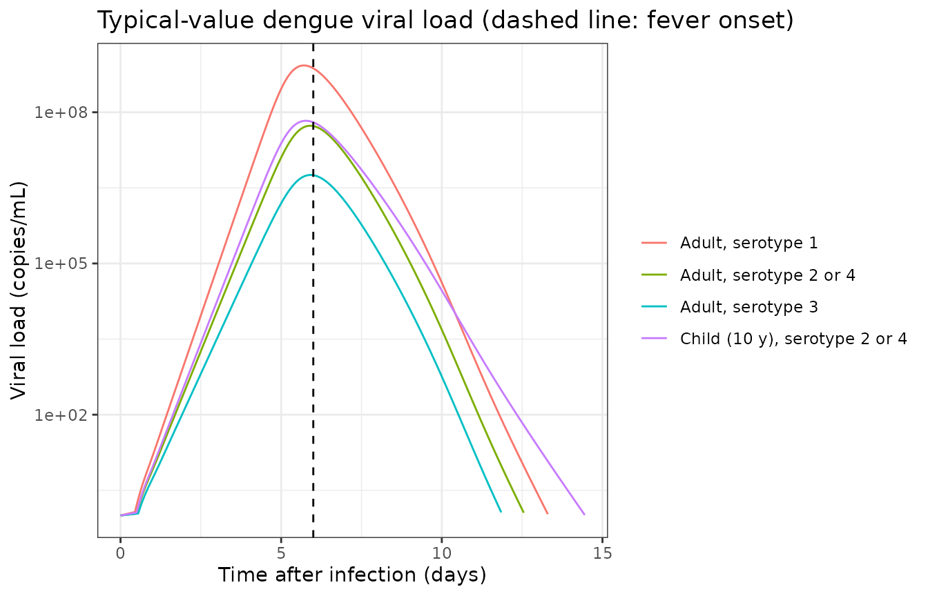
ab <- viral |>
  filter(scenario == "Adult, serotype 2 or 4") |>
  select(time, igm_denv, igg_denv, ab_norm) |>
  tidyr::pivot_longer(-time) |>
  mutate(name = dplyr::recode(name, igm_denv = "IgM", igg_denv = "IgG",
                              ab_norm = "Normalised A(t) x 100"),
         value = ifelse(name == "Normalised A(t) x 100", value * 100, value))
ggplot(ab, aes(time, value, colour = name)) +
  geom_line() +
  labs(x = "Time after infection (days)", y = "Level (assay units)", colour = NULL,
       title = "Typical dengue-specific IgM and IgG (Equations 7-9)") +
  theme_bw()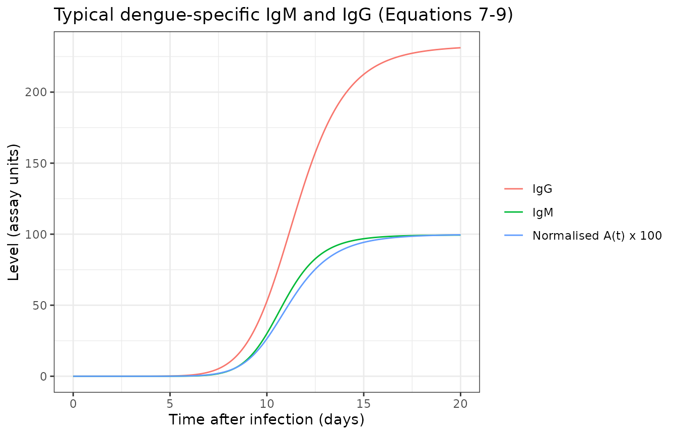
NS1 and the ivermectin dosing scenarios (Figure 4, Table 3, Table S5)
The paper simulated 1000 virtual patients per scenario and reported the median and 95% interval of the per-patient NS1 AUC reduction relative to placebo. Here 200 virtual patients carry the same random effects in every scenario, so each patient’s treated AUC is compared with that patient’s own placebo AUC. The random effects are drawn once with base R from the model’s diagonal omega and passed to the typical-value model as data columns. The AUC is taken over days 0-42 after infection; NS1 has returned to baseline well before day 42, so the window end does not matter.
n_sub <- 200
omega <- rxode2::rxode2(mod)$omega
#> ℹ parameter labels from comments will be replaced by 'label()'
set.seed(20241211)
etas <- as.data.frame(
  sapply(rownames(omega), function(nm) rnorm(n_sub, 0, sqrt(omega[nm, nm])))
)
etas$id <- seq_len(n_sub)

ns1_grid <- seq(0, 42, by = 0.1)

simulate_scenario <- function(dose_days, mgkg, wt, eta_df) {
  obs <- expand.grid(id = eta_df$id, time = ns1_grid)
  obs$amt <- 0
  obs$evid <- 0
  obs$cmt <- "ns1"
  ev <- obs
  if (length(dose_days) > 0) {
    dose <- expand.grid(id = eta_df$id, time = dose_days)
    dose$amt <- mgkg / 1000 * wt
    dose$evid <- 1
    dose$cmt <- "depot"
    ev <- rbind(obs, dose)
  }
  ev <- typical_covariates(ev, wt = wt)
  ev <- merge(ev, eta_df, by = "id")
  ev <- ev[order(ev$id, ev$time, -ev$evid), ]
  s <- solve_typical(ev)
  # rxSolve drops the id column for a single subject
  if (!"id" %in% names(s)) s$id <- eta_df$id[1]
  s[, c("id", "time", "ns1")]
}

scenarios <- tibble::tribble(
  ~scenario,              ~days,         ~dose,
  "Placebo",              numeric(0),    0,
  "Days 7, 8, 9",         c(7, 8, 9),    400,
  "Days 8, 9, 10",        c(8, 9, 10),   400,
  "Days 9, 10, 11",       c(9, 10, 11),  400,
  "Day 7",                7,             400,
  "Days 7, 8",            c(7, 8),       400,
  "Day 8",                8,             400,
  "Days 8, 9",            c(8, 9),       400,
  "Day 7",                7,             600,
  "Day 7",                7,             800,
  "Day 8",                8,             600,
  "Day 8",                8,             800,
  "Days 7, 8",            c(7, 8),       600,
  "Days 7, 8",            c(7, 8),       800
)

run_population <- function(wt, eta_df = etas) {
  dplyr::bind_rows(lapply(seq_len(nrow(scenarios)), function(i) {
    s <- simulate_scenario(scenarios$days[[i]], scenarios$dose[i], wt, eta_df)
    s$scenario <- scenarios$scenario[i]
    s$dose <- scenarios$dose[i]
    s
  }))
}

sim_adult <- run_population(60)
#> ℹ omega/sigma items treated as zero: 'etalcl', 'etalq', 'etalmtt', 'etalfdepot', 'etalbeta', 'etaldelta', 'etalemax_igm', 'etalet50_igm', 'etalhill_igm', 'etalet50_igg', 'etalhill_igg', 'etalktr_ns1', 'etalet50_ns1', 'etalkbase_ns1'
#> ℹ omega/sigma items treated as zero: 'etalcl', 'etalq', 'etalmtt', 'etalfdepot', 'etalbeta', 'etaldelta', 'etalemax_igm', 'etalet50_igm', 'etalhill_igm', 'etalet50_igg', 'etalhill_igg', 'etalktr_ns1', 'etalet50_ns1', 'etalkbase_ns1'
#> ℹ omega/sigma items treated as zero: 'etalcl', 'etalq', 'etalmtt', 'etalfdepot', 'etalbeta', 'etaldelta', 'etalemax_igm', 'etalet50_igm', 'etalhill_igm', 'etalet50_igg', 'etalhill_igg', 'etalktr_ns1', 'etalet50_ns1', 'etalkbase_ns1'
#> ℹ omega/sigma items treated as zero: 'etalcl', 'etalq', 'etalmtt', 'etalfdepot', 'etalbeta', 'etaldelta', 'etalemax_igm', 'etalet50_igm', 'etalhill_igm', 'etalet50_igg', 'etalhill_igg', 'etalktr_ns1', 'etalet50_ns1', 'etalkbase_ns1'
#> ℹ omega/sigma items treated as zero: 'etalcl', 'etalq', 'etalmtt', 'etalfdepot', 'etalbeta', 'etaldelta', 'etalemax_igm', 'etalet50_igm', 'etalhill_igm', 'etalet50_igg', 'etalhill_igg', 'etalktr_ns1', 'etalet50_ns1', 'etalkbase_ns1'
#> ℹ omega/sigma items treated as zero: 'etalcl', 'etalq', 'etalmtt', 'etalfdepot', 'etalbeta', 'etaldelta', 'etalemax_igm', 'etalet50_igm', 'etalhill_igm', 'etalet50_igg', 'etalhill_igg', 'etalktr_ns1', 'etalet50_ns1', 'etalkbase_ns1'
#> ℹ omega/sigma items treated as zero: 'etalcl', 'etalq', 'etalmtt', 'etalfdepot', 'etalbeta', 'etaldelta', 'etalemax_igm', 'etalet50_igm', 'etalhill_igm', 'etalet50_igg', 'etalhill_igg', 'etalktr_ns1', 'etalet50_ns1', 'etalkbase_ns1'
#> ℹ omega/sigma items treated as zero: 'etalcl', 'etalq', 'etalmtt', 'etalfdepot', 'etalbeta', 'etaldelta', 'etalemax_igm', 'etalet50_igm', 'etalhill_igm', 'etalet50_igg', 'etalhill_igg', 'etalktr_ns1', 'etalet50_ns1', 'etalkbase_ns1'
#> ℹ omega/sigma items treated as zero: 'etalcl', 'etalq', 'etalmtt', 'etalfdepot', 'etalbeta', 'etaldelta', 'etalemax_igm', 'etalet50_igm', 'etalhill_igm', 'etalet50_igg', 'etalhill_igg', 'etalktr_ns1', 'etalet50_ns1', 'etalkbase_ns1'
#> ℹ omega/sigma items treated as zero: 'etalcl', 'etalq', 'etalmtt', 'etalfdepot', 'etalbeta', 'etaldelta', 'etalemax_igm', 'etalet50_igm', 'etalhill_igm', 'etalet50_igg', 'etalhill_igg', 'etalktr_ns1', 'etalet50_ns1', 'etalkbase_ns1'
#> ℹ omega/sigma items treated as zero: 'etalcl', 'etalq', 'etalmtt', 'etalfdepot', 'etalbeta', 'etaldelta', 'etalemax_igm', 'etalet50_igm', 'etalhill_igm', 'etalet50_igg', 'etalhill_igg', 'etalktr_ns1', 'etalet50_ns1', 'etalkbase_ns1'
#> ℹ omega/sigma items treated as zero: 'etalcl', 'etalq', 'etalmtt', 'etalfdepot', 'etalbeta', 'etaldelta', 'etalemax_igm', 'etalet50_igm', 'etalhill_igm', 'etalet50_igg', 'etalhill_igg', 'etalktr_ns1', 'etalet50_ns1', 'etalkbase_ns1'
#> ℹ omega/sigma items treated as zero: 'etalcl', 'etalq', 'etalmtt', 'etalfdepot', 'etalbeta', 'etaldelta', 'etalemax_igm', 'etalet50_igm', 'etalhill_igm', 'etalet50_igg', 'etalhill_igg', 'etalktr_ns1', 'etalet50_ns1', 'etalkbase_ns1'
#> ℹ omega/sigma items treated as zero: 'etalcl', 'etalq', 'etalmtt', 'etalfdepot', 'etalbeta', 'etaldelta', 'etalemax_igm', 'etalet50_igm', 'etalhill_igm', 'etalet50_igg', 'etalhill_igg', 'etalktr_ns1', 'etalet50_ns1', 'etalkbase_ns1'
sim_child <- run_population(30)
#> ℹ omega/sigma items treated as zero: 'etalcl', 'etalq', 'etalmtt', 'etalfdepot', 'etalbeta', 'etaldelta', 'etalemax_igm', 'etalet50_igm', 'etalhill_igm', 'etalet50_igg', 'etalhill_igg', 'etalktr_ns1', 'etalet50_ns1', 'etalkbase_ns1'
#> ℹ omega/sigma items treated as zero: 'etalcl', 'etalq', 'etalmtt', 'etalfdepot', 'etalbeta', 'etaldelta', 'etalemax_igm', 'etalet50_igm', 'etalhill_igm', 'etalet50_igg', 'etalhill_igg', 'etalktr_ns1', 'etalet50_ns1', 'etalkbase_ns1'
#> ℹ omega/sigma items treated as zero: 'etalcl', 'etalq', 'etalmtt', 'etalfdepot', 'etalbeta', 'etaldelta', 'etalemax_igm', 'etalet50_igm', 'etalhill_igm', 'etalet50_igg', 'etalhill_igg', 'etalktr_ns1', 'etalet50_ns1', 'etalkbase_ns1'
#> ℹ omega/sigma items treated as zero: 'etalcl', 'etalq', 'etalmtt', 'etalfdepot', 'etalbeta', 'etaldelta', 'etalemax_igm', 'etalet50_igm', 'etalhill_igm', 'etalet50_igg', 'etalhill_igg', 'etalktr_ns1', 'etalet50_ns1', 'etalkbase_ns1'
#> ℹ omega/sigma items treated as zero: 'etalcl', 'etalq', 'etalmtt', 'etalfdepot', 'etalbeta', 'etaldelta', 'etalemax_igm', 'etalet50_igm', 'etalhill_igm', 'etalet50_igg', 'etalhill_igg', 'etalktr_ns1', 'etalet50_ns1', 'etalkbase_ns1'
#> ℹ omega/sigma items treated as zero: 'etalcl', 'etalq', 'etalmtt', 'etalfdepot', 'etalbeta', 'etaldelta', 'etalemax_igm', 'etalet50_igm', 'etalhill_igm', 'etalet50_igg', 'etalhill_igg', 'etalktr_ns1', 'etalet50_ns1', 'etalkbase_ns1'
#> ℹ omega/sigma items treated as zero: 'etalcl', 'etalq', 'etalmtt', 'etalfdepot', 'etalbeta', 'etaldelta', 'etalemax_igm', 'etalet50_igm', 'etalhill_igm', 'etalet50_igg', 'etalhill_igg', 'etalktr_ns1', 'etalet50_ns1', 'etalkbase_ns1'
#> ℹ omega/sigma items treated as zero: 'etalcl', 'etalq', 'etalmtt', 'etalfdepot', 'etalbeta', 'etaldelta', 'etalemax_igm', 'etalet50_igm', 'etalhill_igm', 'etalet50_igg', 'etalhill_igg', 'etalktr_ns1', 'etalet50_ns1', 'etalkbase_ns1'
#> ℹ omega/sigma items treated as zero: 'etalcl', 'etalq', 'etalmtt', 'etalfdepot', 'etalbeta', 'etaldelta', 'etalemax_igm', 'etalet50_igm', 'etalhill_igm', 'etalet50_igg', 'etalhill_igg', 'etalktr_ns1', 'etalet50_ns1', 'etalkbase_ns1'
#> ℹ omega/sigma items treated as zero: 'etalcl', 'etalq', 'etalmtt', 'etalfdepot', 'etalbeta', 'etaldelta', 'etalemax_igm', 'etalet50_igm', 'etalhill_igm', 'etalet50_igg', 'etalhill_igg', 'etalktr_ns1', 'etalet50_ns1', 'etalkbase_ns1'
#> ℹ omega/sigma items treated as zero: 'etalcl', 'etalq', 'etalmtt', 'etalfdepot', 'etalbeta', 'etaldelta', 'etalemax_igm', 'etalet50_igm', 'etalhill_igm', 'etalet50_igg', 'etalhill_igg', 'etalktr_ns1', 'etalet50_ns1', 'etalkbase_ns1'
#> ℹ omega/sigma items treated as zero: 'etalcl', 'etalq', 'etalmtt', 'etalfdepot', 'etalbeta', 'etaldelta', 'etalemax_igm', 'etalet50_igm', 'etalhill_igm', 'etalet50_igg', 'etalhill_igg', 'etalktr_ns1', 'etalet50_ns1', 'etalkbase_ns1'
#> ℹ omega/sigma items treated as zero: 'etalcl', 'etalq', 'etalmtt', 'etalfdepot', 'etalbeta', 'etaldelta', 'etalemax_igm', 'etalet50_igm', 'etalhill_igm', 'etalet50_igg', 'etalhill_igg', 'etalktr_ns1', 'etalet50_ns1', 'etalkbase_ns1'
#> ℹ omega/sigma items treated as zero: 'etalcl', 'etalq', 'etalmtt', 'etalfdepot', 'etalbeta', 'etaldelta', 'etalemax_igm', 'etalet50_igm', 'etalhill_igm', 'etalet50_igg', 'etalhill_igg', 'etalktr_ns1', 'etalet50_ns1', 'etalkbase_ns1'

# Typical-value adult (all random effects 0) for Figure 4
etas_zero <- etas[1, ]
etas_zero[setdiff(names(etas_zero), "id")] <- 0
sim_typical <- run_population(60, etas_zero)
#> ℹ omega/sigma items treated as zero: 'etalcl', 'etalq', 'etalmtt', 'etalfdepot', 'etalbeta', 'etaldelta', 'etalemax_igm', 'etalet50_igm', 'etalhill_igm', 'etalet50_igg', 'etalhill_igg', 'etalktr_ns1', 'etalet50_ns1', 'etalkbase_ns1'
#> ℹ omega/sigma items treated as zero: 'etalcl', 'etalq', 'etalmtt', 'etalfdepot', 'etalbeta', 'etaldelta', 'etalemax_igm', 'etalet50_igm', 'etalhill_igm', 'etalet50_igg', 'etalhill_igg', 'etalktr_ns1', 'etalet50_ns1', 'etalkbase_ns1'
#> ℹ omega/sigma items treated as zero: 'etalcl', 'etalq', 'etalmtt', 'etalfdepot', 'etalbeta', 'etaldelta', 'etalemax_igm', 'etalet50_igm', 'etalhill_igm', 'etalet50_igg', 'etalhill_igg', 'etalktr_ns1', 'etalet50_ns1', 'etalkbase_ns1'
#> ℹ omega/sigma items treated as zero: 'etalcl', 'etalq', 'etalmtt', 'etalfdepot', 'etalbeta', 'etaldelta', 'etalemax_igm', 'etalet50_igm', 'etalhill_igm', 'etalet50_igg', 'etalhill_igg', 'etalktr_ns1', 'etalet50_ns1', 'etalkbase_ns1'
#> ℹ omega/sigma items treated as zero: 'etalcl', 'etalq', 'etalmtt', 'etalfdepot', 'etalbeta', 'etaldelta', 'etalemax_igm', 'etalet50_igm', 'etalhill_igm', 'etalet50_igg', 'etalhill_igg', 'etalktr_ns1', 'etalet50_ns1', 'etalkbase_ns1'
#> ℹ omega/sigma items treated as zero: 'etalcl', 'etalq', 'etalmtt', 'etalfdepot', 'etalbeta', 'etaldelta', 'etalemax_igm', 'etalet50_igm', 'etalhill_igm', 'etalet50_igg', 'etalhill_igg', 'etalktr_ns1', 'etalet50_ns1', 'etalkbase_ns1'
#> ℹ omega/sigma items treated as zero: 'etalcl', 'etalq', 'etalmtt', 'etalfdepot', 'etalbeta', 'etaldelta', 'etalemax_igm', 'etalet50_igm', 'etalhill_igm', 'etalet50_igg', 'etalhill_igg', 'etalktr_ns1', 'etalet50_ns1', 'etalkbase_ns1'
#> ℹ omega/sigma items treated as zero: 'etalcl', 'etalq', 'etalmtt', 'etalfdepot', 'etalbeta', 'etaldelta', 'etalemax_igm', 'etalet50_igm', 'etalhill_igm', 'etalet50_igg', 'etalhill_igg', 'etalktr_ns1', 'etalet50_ns1', 'etalkbase_ns1'
#> ℹ omega/sigma items treated as zero: 'etalcl', 'etalq', 'etalmtt', 'etalfdepot', 'etalbeta', 'etaldelta', 'etalemax_igm', 'etalet50_igm', 'etalhill_igm', 'etalet50_igg', 'etalhill_igg', 'etalktr_ns1', 'etalet50_ns1', 'etalkbase_ns1'
#> ℹ omega/sigma items treated as zero: 'etalcl', 'etalq', 'etalmtt', 'etalfdepot', 'etalbeta', 'etaldelta', 'etalemax_igm', 'etalet50_igm', 'etalhill_igm', 'etalet50_igg', 'etalhill_igg', 'etalktr_ns1', 'etalet50_ns1', 'etalkbase_ns1'
#> ℹ omega/sigma items treated as zero: 'etalcl', 'etalq', 'etalmtt', 'etalfdepot', 'etalbeta', 'etaldelta', 'etalemax_igm', 'etalet50_igm', 'etalhill_igm', 'etalet50_igg', 'etalhill_igg', 'etalktr_ns1', 'etalet50_ns1', 'etalkbase_ns1'
#> ℹ omega/sigma items treated as zero: 'etalcl', 'etalq', 'etalmtt', 'etalfdepot', 'etalbeta', 'etaldelta', 'etalemax_igm', 'etalet50_igm', 'etalhill_igm', 'etalet50_igg', 'etalhill_igg', 'etalktr_ns1', 'etalet50_ns1', 'etalkbase_ns1'
#> ℹ omega/sigma items treated as zero: 'etalcl', 'etalq', 'etalmtt', 'etalfdepot', 'etalbeta', 'etaldelta', 'etalemax_igm', 'etalet50_igm', 'etalhill_igm', 'etalet50_igg', 'etalhill_igg', 'etalktr_ns1', 'etalet50_ns1', 'etalkbase_ns1'
#> ℹ omega/sigma items treated as zero: 'etalcl', 'etalq', 'etalmtt', 'etalfdepot', 'etalbeta', 'etaldelta', 'etalemax_igm', 'etalet50_igm', 'etalhill_igm', 'etalet50_igg', 'etalhill_igg', 'etalktr_ns1', 'etalet50_ns1', 'etalkbase_ns1'

auc_reduction <- function(sim) {
  auc <- sim |>
    group_by(scenario, dose, id) |>
    summarise(auc = sum(diff(time) * (head(ns1, -1) + tail(ns1, -1)) / 2), .groups = "drop")
  placebo <- auc |> filter(scenario == "Placebo") |> select(id, auc_placebo = auc)
  auc |>
    filter(scenario != "Placebo") |>
    left_join(placebo, by = "id") |>
    mutate(reduction = 100 * (1 - auc / auc_placebo)) |>
    group_by(scenario, dose) |>
    summarise(
      median = median(reduction),
      lo = quantile(reduction, 0.025),
      hi = quantile(reduction, 0.975),
      .groups = "drop"
    )
}
Figure 4: NS1 profiles in a typical adult
Figure 4 is captioned as the simulated median profile, but its placebo curve (peak about 1300 ng/mL at about day 8.7) matches the typical-value profile, i.e. the profile with all random effects at zero. The cross-sectional median of the virtual patients is lower and later, because the IIV on ET50,NS1 and on the NS1 transit rate spreads the individual peaks over several days. The figure is therefore replicated with typical values, and the cross-sectional median is reported for comparison below the plot.
panel_def <- list(
  "(a) 400 ug/kg x 3 days, start day" = list(c("Placebo", 0), c("Days 7, 8, 9", 400), c("Days 8, 9, 10", 400), c("Days 9, 10, 11", 400)),
  "(b) 400 ug/kg, duration from day 7" = list(c("Placebo", 0), c("Day 7", 400), c("Days 7, 8", 400), c("Days 7, 8, 9", 400)),
  "(c) 400 ug/kg, duration from day 8" = list(c("Placebo", 0), c("Day 8", 400), c("Days 8, 9", 400), c("Days 8, 9, 10", 400)),
  "(d) dose, day 7" = list(c("Placebo", 0), c("Day 7", 400), c("Day 7", 600), c("Day 7", 800)),
  "(e) dose, day 8" = list(c("Placebo", 0), c("Day 8", 400), c("Day 8", 600), c("Day 8", 800)),
  "(f) dose, days 7 and 8" = list(c("Placebo", 0), c("Days 7, 8", 400), c("Days 7, 8", 600), c("Days 7, 8", 800))
)
typical_profiles <- sim_typical |>
  filter(time <= 21)
fig4 <- dplyr::bind_rows(lapply(names(panel_def), function(p) {
  keys <- do.call(rbind, panel_def[[p]])
  dplyr::bind_rows(lapply(seq_len(nrow(keys)), function(k) {
    typical_profiles |>
      filter(scenario == keys[k, 1], dose == as.numeric(keys[k, 2])) |>
      mutate(panel = p, arm = ifelse(scenario == "Placebo", "Placebo",
                                     paste0(scenario, ", ", dose, " ug/kg/d")))
  }))
}))
ggplot(fig4, aes(time, ns1, colour = arm)) +
  geom_line() +
  facet_wrap(~panel, ncol = 3) +
  labs(x = "Time after infection (days)", y = "NS1 (ng/mL)", colour = NULL,
       title = "Replicates Figure 4 of Ding 2024 (typical adult, 60 kg)") +
  theme_bw() +
  theme(legend.position = "bottom", legend.text = element_text(size = 7)) +
  guides(colour = guide_legend(ncol = 3))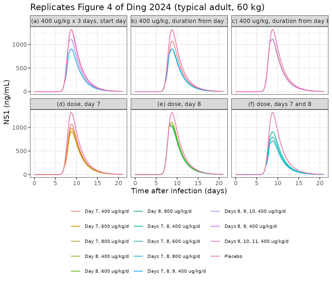
placebo_typical <- typical_profiles |> filter(scenario == "Placebo")
placebo_peak <- max(placebo_typical$ns1)
placebo_tpeak <- placebo_typical$time[which.max(placebo_typical$ns1)]
placebo_median <- sim_adult |>
  filter(scenario == "Placebo") |>
  group_by(time) |>
  summarise(ns1 = median(ns1))
c(
  typical_peak_ng_ml = placebo_peak,
  typical_peak_day = placebo_tpeak,
  median_peak_ng_ml = max(placebo_median$ns1),
  median_peak_day = placebo_median$time[which.max(placebo_median$ns1)]
)
#> typical_peak_ng_ml   typical_peak_day  median_peak_ng_ml    median_peak_day
#>          1317.0218             8.8000           916.9767             9.3000
stopifnot(
  # Figure 4 placebo: about 1300 ng/mL at about day 8.7 (read from the figure)
  abs(placebo_peak / 1300 - 1) < 0.1,
  abs(placebo_tpeak - 8.7) < 0.3
)
The typical placebo profile peaks at 1317 ng/mL on day 8.8; Figure 4 shows a peak of about 1300 ng/mL at about day 8.7.
Table 3 (typical adult) and Table S5 (typical child)
published <- tibble::tribble(
  ~scenario,        ~dose, ~adult_pub,         ~child_pub,
  "Days 7, 8, 9",   400,   "27.8 (7.0-52.2)",  "28.6 (7.3-53.4)",
  "Days 8, 9, 10",  400,   "17.3 (0.7-45.6)",  "17.8 (0.7-46.7)",
  "Days 9, 10, 11", 400,   "4.8 (0.03-36.4)",  "5.0 (0.03-36.5)",
  "Day 7",          400,   "14.1 (4.0-30.0)",  "14.6 (4.2-30.8)",
  "Days 7, 8",      400,   "23.3 (6.5-46.2)",  "24.0 (6.7-46.5)",
  "Day 8",          400,   "11.0 (0.6-29.2)",  "11.5 (0.7-28.9)",
  "Days 8, 9",      400,   "15.8 (0.7-40.5)",  "16.5 (0.7-41.3)",
  "Day 7",          600,   "19.2 (5.6-37.5)",  "19.8 (5.9-38.1)",
  "Day 7",          800,   "23.3 (7.2-43.2)",  "24.1 (7.3-44.0)",
  "Day 8",          600,   "14.7 (0.8-36.0)",  "15.1 (0.8-36.4)",
  "Day 8",          800,   "17.7 (0.9-41.5)",  "18.3 (1.0-42.2)",
  "Days 7, 8",      600,   "30.2 (8.5-54.8)",  "30.9 (9.0-55.4)",
  "Days 7, 8",      800,   "35.5 (9.9-60.8)",  "36.3 (10.3-61.2)"
) |>
  mutate(
    adult_pub_median = as.numeric(sub(" .*", "", adult_pub)),
    child_pub_median = as.numeric(sub(" .*", "", child_pub))
  )

fmt <- function(m, lo, hi) sprintf("%.1f (%.1f-%.1f)", m, lo, hi)
red_adult <- auc_reduction(sim_adult) |> mutate(adult_sim = fmt(median, lo, hi), adult_sim_median = median)
red_child <- auc_reduction(sim_child) |> mutate(child_sim = fmt(median, lo, hi), child_sim_median = median)

cmp <- published |>
  left_join(red_adult |> select(scenario, dose, adult_sim, adult_sim_median), by = c("scenario", "dose")) |>
  left_join(red_child |> select(scenario, dose, child_sim, child_sim_median), by = c("scenario", "dose"))

cmp |>
  select(scenario, dose, adult_pub, adult_sim, child_pub, child_sim) |>
  dplyr::rename(
    "Ivermectin dosing (day after infection)" = scenario,
    "Dose (ug/kg/day)" = dose,
    "Adult, Table 3" = adult_pub,
    "Adult, simulated" = adult_sim,
    "Child, Table S5" = child_pub,
    "Child, simulated" = child_sim
  ) |>
  knitr::kable(caption = paste(
    "NS1 AUC reduction relative to placebo, median % (95% interval).",
    "Published: 1000 virtual patients per scenario; simulated: 200."
))| Ivermectin dosing (day after infection) | Dose (ug/kg/day) | Adult, Table 3 | Adult, simulated | Child, Table S5 | Child, simulated |
|---|---|---|---|---|---|
| Days 7, 8, 9 | 400 | 27.8 (7.0-52.2) | 28.8 (11.3-50.4) | 28.6 (7.3-53.4) | 29.0 (11.9-52.4) |
| Days 8, 9, 10 | 400 | 17.3 (0.7-45.6) | 15.5 (1.5-42.8) | 17.8 (0.7-46.7) | 16.1 (1.6-43.9) |
| Days 9, 10, 11 | 400 | 4.8 (0.03-36.4) | 3.8 (0.1-31.5) | 5.0 (0.03-36.5) | 4.0 (0.1-32.5) |
| Day 7 | 400 | 14.1 (4.0-30.0) | 15.3 (4.4-29.1) | 14.6 (4.2-30.8) | 15.7 (4.5-30.3) |
| Days 7, 8 | 400 | 23.3 (6.5-46.2) | 24.0 (8.4-42.9) | 24.0 (6.7-46.5) | 24.8 (8.4-44.4) |
| Day 8 | 400 | 11.0 (0.6-29.2) | 11.0 (1.4-28.9) | 11.5 (0.7-28.9) | 11.4 (1.4-29.7) |
| Days 8, 9 | 400 | 15.8 (0.7-40.5) | 14.7 (1.5-40.7) | 16.5 (0.7-41.3) | 15.1 (1.6-42.1) |
| Day 7 | 600 | 19.2 (5.6-37.5) | 20.5 (6.4-36.8) | 19.8 (5.9-38.1) | 21.0 (6.5-37.8) |
| Day 7 | 800 | 23.3 (7.2-43.2) | 25.0 (8.0-42.6) | 24.1 (7.3-44.0) | 25.4 (8.0-43.4) |
| Day 8 | 600 | 14.7 (0.8-36.0) | 14.1 (1.7-35.7) | 15.1 (0.8-36.4) | 14.5 (1.7-37.2) |
| Day 8 | 800 | 17.7 (0.9-41.5) | 17.1 (1.9-41.2) | 18.3 (1.0-42.2) | 17.4 (1.9-42.8) |
| Days 7, 8 | 600 | 30.2 (8.5-54.8) | 31.7 (10.6-52.5) | 30.9 (9.0-55.4) | 32.2 (11.2-54.1) |
| Days 7, 8 | 800 | 35.5 (9.9-60.8) | 37.8 (13.5-59.2) | 36.3 (10.3-61.2) | 37.8 (14.2-60.8) |
stopifnot(
  # A wrong EC50, dose unit or NS1 secretion parameter moves every scenario by
  # many percentage points.
  max(abs(cmp$adult_sim_median - cmp$adult_pub_median)) < 5,
  max(abs(cmp$child_sim_median - cmp$child_pub_median)) < 5,
  # Earlier start, longer course and higher dose all give larger reductions.
  with(red_adult, median[scenario == "Days 7, 8, 9"] > median[scenario == "Days 8, 9, 10"]),
  with(red_adult, median[scenario == "Days 8, 9, 10"] > median[scenario == "Days 9, 10, 11"]),
  with(red_adult, median[scenario == "Days 7, 8" & dose == 800] > median[scenario == "Days 7, 8" & dose == 400])
)
Ivermectin PK: PKNCA against Supplementary Table S3
Table S3 reports the median of the individual post hoc Cmax, AUC0-inf and terminal half-life in each study arm. The virtual cohorts below have log-normally distributed body weights matching the Table S2 medians and ranges (200 adults per adult arm, 100 children per paediatric arm). Time is converted to hours for PKNCA. AUC0-inf covers the whole 2- or 3-day course. The paediatric arms in the study had only 12 children each (6 per weight stratum), so their published medians are less precise than the adult ones.
set.seed(20241212)
draw_wt <- function(n, median, lo, hi, sdlog) {
  pmin(pmax(exp(rnorm(n, log(median), sdlog)), lo), hi)
}
pk_grid <- sort(unique(c(seq(0, 4, by = 0.02), seq(4, 40, by = 0.25))))
pk_arms <- tibble::tribble(
  ~treatment,                  ~n,  ~ndose, ~mgkg, ~wt_med, ~wt_lo, ~wt_hi, ~sdlog,
  "Adult 400 ug/kg x 2 days",  200, 2,      400,   60,      35,     135,    0.2,
  "Adult 400 ug/kg x 3 days",  200, 3,      400,   60,      35,     135,    0.2,
  "Child 400 ug/kg x 3 days",  100, 3,      400,   29.9,    17.2,   69.1,   0.3,
  "Child 600 ug/kg x 3 days",  100, 3,      600,   29.9,    17.2,   69.1,   0.3
)
pk_events <- dplyr::bind_rows(lapply(seq_len(nrow(pk_arms)), function(i) {
  a <- pk_arms[i, ]
  ids <- (i - 1) * 1000 + seq_len(a$n)
  wt <- draw_wt(a$n, a$wt_med, a$wt_lo, a$wt_hi, a$sdlog)
  obs <- data.frame(id = rep(ids, each = length(pk_grid)), time = rep(pk_grid, a$n),
                    amt = 0, evid = 0, cmt = "ns1")
  dose <- data.frame(id = rep(ids, each = a$ndose), time = rep(seq_len(a$ndose) - 1, a$n),
                     amt = rep(a$mgkg / 1000 * wt, each = a$ndose), evid = 1, cmt = "depot")
  ev <- rbind(obs, dose)
  ev$WT <- wt[match(ev$id, ids)]
  ev$treatment <- a$treatment
  ev
}))
# Time is shifted so the first dose is at time 0; the antibody and NS1 time
# courses do not feed back on ivermectin PK.
pk_events <- typical_covariates(pk_events, wt = pk_events$WT)
pk_events <- pk_events[order(pk_events$id, pk_events$time, -pk_events$evid), ]
pk_sim <- as.data.frame(rxode2::rxSolve(mod, pk_events, keep = "treatment",
                                        returnType = "data.frame"))
#> ℹ parameter labels from comments will be replaced by 'label()'
conc <- pk_sim |>
  filter(!is.na(Cc)) |>
  mutate(time_h = time * 24) |>
  select(id, treatment, time_h, Cc)
conc_obj <- PKNCA::PKNCAconc(conc, Cc ~ time_h | treatment + id)
intervals <- data.frame(start = 0, end = Inf, cmax = TRUE, tmax = TRUE,
                        aucinf.obs = TRUE, half.life = TRUE)
nca <- PKNCA::pk.nca(PKNCA::PKNCAdata(conc_obj, intervals = intervals))
#> No dose information provided, calculations requiring dose will return NA.

reference <- tibble::tribble(
  ~treatment,                 ~cmax, ~aucinf.obs, ~half.life,
  "Adult 400 ug/kg x 2 days", 77.8,  4490,        94.2,
  "Adult 400 ug/kg x 3 days", 82.1,  5700,        94.2,
  "Child 400 ug/kg x 3 days", 120,   6900,        83.6,
  "Child 600 ug/kg x 3 days", 177,   11900,       83.6
)
pk_cmp <- nlmixr2lib::ncaComparisonTable(
  simulated = nca,
  reference = reference,
  by = "treatment",
  params = c("cmax", "aucinf.obs", "half.life"),
  units = c(cmax = "ng/mL", aucinf.obs = "ng*h/mL", half.life = "h"),
  tolerance_pct = 20
)
pk_cmp |>
  dplyr::rename("Arm" = treatment) |>
  knitr::kable(caption = paste(
    "Simulated ivermectin NCA (median) versus Supplementary Table S3 medians.",
    "Half-life is reported per age group in Table S3, so the same value is",
    "shown for both arms of a group.",
    attr(pk_cmp, "footnote")
))| NCA parameter | Arm | Reference | Simulated | % diff |
|---|---|---|---|---|
| Cmax (ng/mL) | Adult 400 ug/kg x 2 days | 77.8 | 76.2 | -2.1% |
| Cmax (ng/mL) | Adult 400 ug/kg x 3 days | 82.1 | 80.4 | -2.1% |
| Cmax (ng/mL) | Child 400 ug/kg x 3 days | 120 | 107 | -10.8% |
| Cmax (ng/mL) | Child 600 ug/kg x 3 days | 177 | 148 | -16.2% |
| AUC0-∞ (obs) (ng*h/mL) | Adult 400 ug/kg x 2 days | 4490 | 4120 | -8.2% |
| AUC0-∞ (obs) (ng*h/mL) | Adult 400 ug/kg x 3 days | 5700 | 5780 | +1.4% |
| AUC0-∞ (obs) (ng*h/mL) | Child 400 ug/kg x 3 days | 6900 | 6240 | -9.6% |
| AUC0-∞ (obs) (ng*h/mL) | Child 600 ug/kg x 3 days | 11900 | 9460 | -20.5%* |
| t½ (h) | Adult 400 ug/kg x 2 days | 94.2 | 94.7 | +0.6% |
| t½ (h) | Adult 400 ug/kg x 3 days | 94.2 | 96.3 | +2.2% |
| t½ (h) | Child 400 ug/kg x 3 days | 83.6 | 71.2 | -14.8% |
| t½ (h) | Child 600 ug/kg x 3 days | 83.6 | 71.9 | -14.0% |
nca_med <- as.data.frame(nca$result) |>
  group_by(treatment, PPTESTCD) |>
  summarise(med = median(PPORRES, na.rm = TRUE), .groups = "drop") |>
  tidyr::pivot_wider(names_from = PPTESTCD, values_from = med) |>
  left_join(reference, by = "treatment", suffix = c("", "_pub"))
stopifnot(
  all(abs(nca_med$cmax / nca_med$cmax_pub - 1) < 0.25),
  all(abs(nca_med$aucinf.obs / nca_med$aucinf.obs_pub - 1) < 0.30)
)
pk_sim |>
  group_by(treatment, time) |>
  summarise(med = median(Cc), lo = quantile(Cc, 0.05), hi = quantile(Cc, 0.95),
            .groups = "drop") |>
  filter(time <= 10) |>
  ggplot(aes(time * 24, med, colour = treatment, fill = treatment)) +
  geom_ribbon(aes(ymin = lo, ymax = hi), alpha = 0.15, colour = NA) +
  geom_line() +
  labs(x = "Time after first dose (h)", y = "Ivermectin (ng/mL)", colour = NULL, fill = NULL,
       title = "Simulated ivermectin concentrations (median, 90% interval)") +
  theme_bw()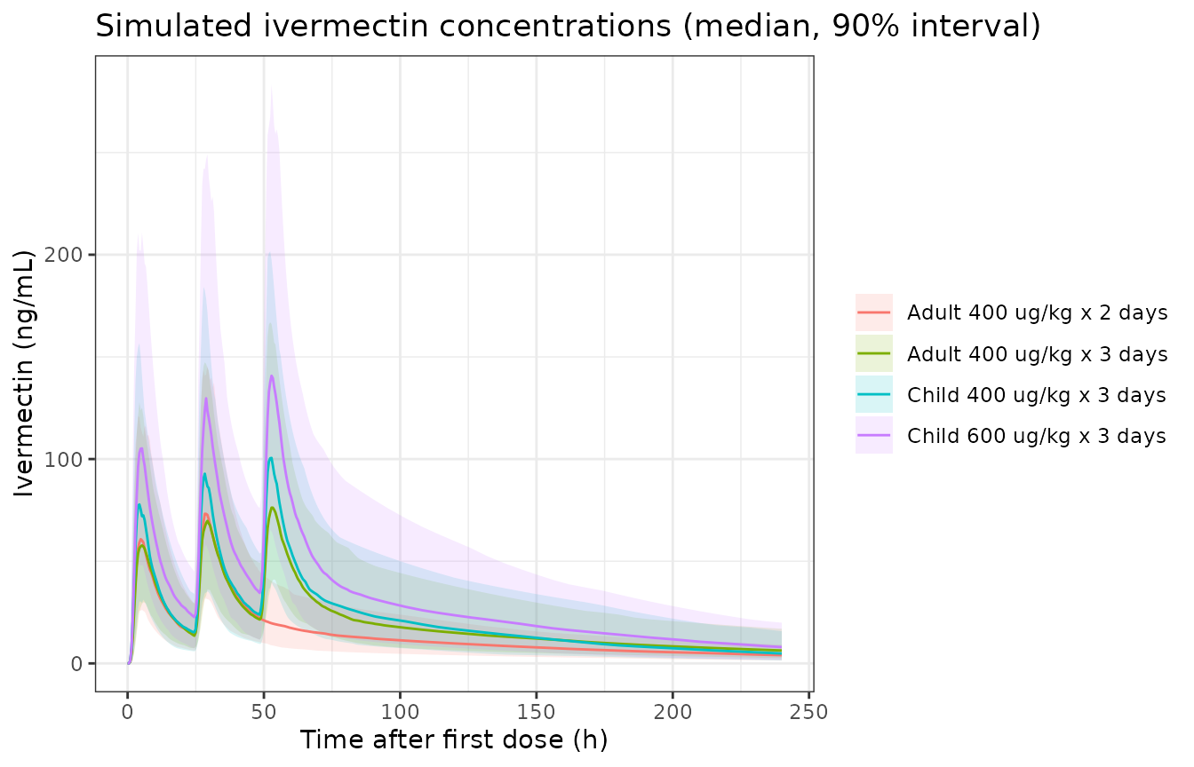
Assumptions and deviations
-
NS1 KTR and Emax,NS1. The NS1 NONMEM code in the
supplement labels
THETA(5)(initial 6.76) as the maximum NS1 secretion rate andTHETA(6)(initial 1.02) as the NS1 transit rate, whereas Table 2 gives KTR = 6.76 (with IIV 37.9%) and Emax,NS1 = 1.04. The code reading gives an NS1 peak of about 2e5 ng/mL near day 15, far from Figure 4; the Table 2 reading reproduces Figure 4 and Table 3, so Table 2 is used. -
Serotype effects. The Table 1 note describes
categorical covariates as a proportional effect on the parameter, but
the viral NONMEM code applies the serotype factor to the log10 exponent
(
TVBETA = THETA(1) * CSERO1; BETA = 10**TVBETA, and likewise for p). The code form is used. It gives the ordering stated in the Discussion (serotype 1 higher, serotype 3 lower viral loads); a linear factor of 1.15 on beta would barely change the viral load. - T0. Table 1 prints T0 = 3.5 x 10^6 cells/mL; the Methods, the Figure 1 legend and both NONMEM codes give 3.5 x 10^5 cells/mL, which is used.
-
Number of PK transit compartments. The PK control
stream sets
NN = 7, but the text, the Figure 1 legend, Table S3 and the NS1 control stream (which carries the final PK model into the PK-PD fit) all use 6 transit compartments withKTR = (NN + 1) / MT. Six compartments and ktr = 7 / MTT are used. -
NS1-specific IgG slope. Table 2 gives 0.112; its
footnote prints 0.108. The table value is used. The IgG enters as
max(log(ABNS1_IGG) - 4, 0), so the covariate column holds the linear relative-unit level (the source dataset columnIGGNholds its natural log), and the IIV on kbase multiplies the whole elimination rate, as in the NONMEM code. -
Age covariates. Both age effects are linear splines
that apply only below 20 years (
min(AGE, 20) - 20). The NONMEM$INPUTcomments label AGE as months, but the 20-year cut-off in the text and tables is in years. Table 1 rounds the age effect on delta to 2.5%; the code and Supplementary Results give 2.52%, which is used. -
Residual error. The viral-load and NS1 residual
errors (1.31 and 1.15) equal the NONMEM
$SIGMAestimates, so they are variances and the model uses their square roots as the log-scale SD. The PK, IgM and IgG residual errors are reported as percentages and are used as log-scale SDs. -
Neutralisation term. Equation 10 prints
dV/dt = pP - cV - kA A; the NONMEM code isKA * HEFF * A(4), i.e. kA x A(t) x V, which is used. -
Infected-cell chain. The text describes three
transit compartments between infected and producing cells; with the
infected compartment itself this gives four compartments before the
producing cells (
eclipse1toeclipse4), as in the NONMEM code. - IIV on IgG Emax. Table S4 reports no IIV on the IgG Emax, so A(t) uses the typical IgG Emax; IIV on the IgM Emax cancels in the normalised A(t).
- Units. The abstract gives the ivermectin EC50 as 67.5 ug/mL; Table 2 and the plasma concentrations (Cmax around 80 ng/mL) show it is 67.5 ng/mL. Table S3 labels AUC as ug.h/mL; the values (around 5700) are ng.h/mL.
- Typical patients. The typical age and anti-NS1 IgG are not stated; see “Typical patients” above. The paediatric scenarios use an age of 25 years because the paper’s typical child differs from the typical adult only in body weight. The AUC window of Table 3 (“AUC0-42”) is taken as days 0-42 after infection.
- Figure 4. The caption calls the curves simulated medians, but the placebo curve matches the typical-value profile (all random effects zero), not the cross-sectional median of a simulated cohort, which peaks lower and later. The figure is replicated with typical values. Table 3 and Table S5, which report the median and 95% interval of per-patient reductions, are replicated with a 200-patient cohort.
- Not replicated. The viral-load and NS1 visual predictive checks (Figures 2 and 3) need the observed data and the individual enrolment times, which are not published.