S(-)-atenolol and isoprenaline-induced tachycardia in rats (van Steeg 2007)
Source:vignettes/articles/vanSteeg_2007_atenolol_isoprenaline_rat.Rmd
vanSteeg_2007_atenolol_isoprenaline_rat.RmdModel and source
van Steeg and colleagues set out to validate a pharmacodynamic endpoint, not to characterise a drug: they asked whether the reduction of isoprenaline-induced tachycardia is a better readout for beta-blockers in the rat than the reduction of resting heart rate. Answering that required three separately fitted models, so this paper contributes three model files.
- Isoprenaline: Preclinical (rat). Two-compartment micro-constant IV PK of the beta-adrenoceptor agonist isoprenaline in conscious male Wistar-Kyoto (WKY) rats, linked to a DIRECT (no effect compartment) sigmoid Emax model for the resulting increase in heart rate. Isoprenaline is so potent that a maximal chronotropic response occurs at plasma concentrations below the assay limit of quantification, so the PK and the PD were run as SEPARATE experiments and the PD-experiment plasma concentrations were predicted from this PK model rather than measured. This model supplies the tachycardia background against which the companion S(-)-atenolol models were built: modellib(‘vanSteeg_2007_atenolol_iso_rat’) and modellib(‘vanSteeg_2007_atenolol_noniso_rat’). Note the two non-standard variability scales, both taken verbatim from the paper: PK inter-individual variability is EXPONENTIAL (Equation 1) whereas PD inter-individual variability is ADDITIVE in beats/min (Equation 5), and the PD residual error is additive in beats/min despite the paper’s Equation 6 printing a proportional form (see the ini() notes).
- S(-)-atenolol, isoprenaline group: Preclinical (rat). Three-compartment IV-infusion PK of S(-)-atenolol in conscious male Wistar-Kyoto (WKY) rats linked, through an effect compartment, to a sigmoid Emax model for the REDUCTION of isoprenaline-induced tachycardia (heart rate, beats/min). This is the ISOPRENALINE group: tachycardia was maintained by a continuous 5 ug/kg/h IV infusion of isoprenaline started at least 30 min before the atenolol dose, so the baseline E0 = 517 beats/min is the isoprenaline-elevated heart rate and no isoprenaline PK is needed to use this model. The counter-clockwise hysteresis between plasma concentration and effect is resolved by an effect compartment with ke0 = 0.042 1/min (equilibration half-life 16.5 min). The PK was fitted jointly across the isoprenaline and non-isoprenaline groups (no PK difference was found), so the six PK parameters are shared with the companion model modellib(‘vanSteeg_2007_atenolol_noniso_rat’); only the PD differs. Note the two non-standard variability scales, both taken verbatim from the paper: PK inter-individual variability is EXPONENTIAL (Equation 1) whereas PD inter-individual variability is ADDITIVE in beats/min (Equation 5), and the PD residual error is additive in beats/min despite the paper’s Equation 6 printing a proportional form (see the ini() notes).
- S(-)-atenolol, non-isoprenaline group: Preclinical (rat). Three-compartment IV-infusion PK of S(-)-atenolol in conscious male Wistar-Kyoto (WKY) rats linked to a DIRECT-effect Emax model for the reduction of RESTING heart rate (beats/min). This is the NON-ISOPRENALINE (vehicle) group – the negative control for the companion isoprenaline-tachycardia model modellib(‘vanSteeg_2007_atenolol_iso_rat’). It is deliberately the paper’s UNDER-DETERMINED arm and is packaged as such: the drug effect on resting heart rate (Emax = -43 beats/min) is barely larger than the ~30 beats/min spontaneous variation in rat heart rate, so EC50 is estimated with 97% RSE, and neither a Hill coefficient nor an effect-compartment ke0 could be estimated at all – n is FIXED at 1 and there is NO effect compartment, unlike the isoprenaline arm. The PK was fitted jointly across both groups (no PK difference was found), so the six PK parameters are identical to those of the isoprenaline model; only the PD differs. Note the two non-standard variability scales, both taken verbatim from the paper: PK inter-individual variability is EXPONENTIAL (Equation 1) whereas PD inter-individual variability is ADDITIVE in beats/min (Equation 5), and the PD residual error is additive in beats/min despite the paper’s Equation 6 printing a proportional form (see the ini() notes).
- Citation: van Steeg TJ, Freijer J, Danhof M, de Lange ECM. Pharmacokinetic-pharmacodynamic modelling of S(-)-atenolol in rats: reduction of isoprenaline-induced tachycardia as a continuous pharmacodynamic endpoint. British Journal of Pharmacology. 2007;151(3):356-366. doi:10.1038/sj.bjp.0707234. PMCID: PMC2013984. Isoprenaline PK parameters are Table 1; isoprenaline PD parameters are Table 2. Companion model files from the same paper: modellib(‘vanSteeg_2007_atenolol_iso_rat’), modellib(‘vanSteeg_2007_atenolol_noniso_rat’).
- Article: https://doi.org/10.1038/sj.bjp.0707234
- Open-access full text: https://www.ncbi.nlm.nih.gov/pmc/articles/PMC2013984/
Why three files rather than one, or two:
- The isoprenaline model is a self-contained PK-PD model of the agonist, fitted on its own animals in its own experiments (Tables 1 and 2).
- The two S(-)-atenolol models share one PK fit but two independent PD fits. The PK was pooled – “The concentration-time profiles of S(-)-atenolol with and without isoprenaline-induced tachycardia were analysed simultaneously as no differences were found in the PK between both groups” – while the PD was not: “In contrast to the PK data, the PD data were analysed separately, since the baseline heart rate differed between the isoprenaline and the non-isoprenaline group.” Two separate fits give two model files, and they differ structurally as well as numerically: only the isoprenaline arm supports an effect compartment and an estimated Hill coefficient.
iso  <- rxode2::rxode2(readModelDb("vanSteeg_2007_isoprenaline_rat"))
#> ℹ parameter labels from comments will be replaced by 'label()'
aten_iso    <- rxode2::rxode2(readModelDb("vanSteeg_2007_atenolol_iso_rat"))
#> ℹ parameter labels from comments will be replaced by 'label()'
aten_noniso <- rxode2::rxode2(readModelDb("vanSteeg_2007_atenolol_noniso_rat"))
#> ℹ parameter labels from comments will be replaced by 'label()'
Population
Male Wistar-Kyoto (WKY) rats, 294 g +/- 49, housed individually and acclimatised for at least five days, were instrumented seven days before the experiment with four indwelling cannulas: two in the right jugular vein for drug administration, and one in each femoral artery for blood sampling and for heart rate. All experiments began between 08:00 and 09:00 to avoid circadian influences, and the animals were conscious throughout. Thirty-nine rats contributed to this study’s own experiments (Methods, Animals).
The S(-)-atenolol experiment used two groups given the same 5 mg/kg 15-minute intravenous infusion: nine rats on a background of continuous intravenous isoprenaline at 5 ug/kg/h, and eight on vehicle alone (0.1% w/w sodium metabisulphite in saline). The background infusion started at least 30 minutes before the atenolol dose. Arterial samples for plasma S(-)-atenolol were drawn at eighteen times out to 480 minutes; heart rate was recorded continuously.
Isoprenaline was characterised separately because it is too potent to measure and observe at the same time – “a maximal increase in heart rate in rats is obtained with plasma concentrations below the limit of quantification”. Its PK came from fourteen rats given 25 or 50 ug/kg over 10 minutes; its PD came from six rats stepped through eight continuous infusion rates from 0.001 to 2.5 ug/kg/h, supplemented by 17 and 8 rats at 5 and 10 ug/kg/h drawn from other experiments. The PD was therefore fitted against model-predicted, not measured, plasma concentrations.
The same information is available programmatically via each model’s
population metadata (for example
readModelDb("vanSteeg_2007_atenolol_iso_rat")()$population).
Dose scale: the typical 294 g rat
All three models fit absolute volumes (mL) and
absolute clearances or micro-constants, so converting the reported mg/kg
and ug/kg doses into an event-table amt needs a body
weight. Unlike some preclinical papers this one states it: the
Discussion computes an isoprenaline steady state for “a typical rat
of 294 g”, which is also the mean of the Methods weight range.
Every simulation below doses that animal.
WT_KG <- 0.294  # typical rat, van Steeg 2007 Discussion and Methods/Animals

# S(-)-atenolol 5 mg/kg over 15 min, expressed in ng (units$dosing).
ATEN_AMT <- 5 * WT_KG * 1e6   # ng
ATEN_DUR <- 15                # min

# Isoprenaline PK experiment: 25 and 50 ug/kg over 10 min, in ng.
ISO_AMT <- c("25 ug/kg" = 25 * WT_KG * 1e3, "50 ug/kg" = 50 * WT_KG * 1e3)
ISO_DUR <- 10                 # min

c(ATEN_AMT = ATEN_AMT, ISO_AMT)
#> ATEN_AMT 25 ug/kg 50 ug/kg
#>  1470000     7350    14700
Source trace
Every ini() entry in all three model files carries an
in-file comment naming its source location. They are collected here for
review.
| Model | Equation / parameter | Value | Source location |
|---|---|---|---|
| all | Exponential PK IIV, P_i = theta * exp(eta_i)
|
n/a | Equation 1 |
| all | Proportional PK residual,
C_obs = C_pred * (1 + eps)
|
n/a | Equation 2 |
| all | Sigmoid Emax, E = E0 + Emax * C^n / (EC50^n + C^n)
|
n/a | Equation 3 |
| atenolol ISO | Effect compartment, dCe/dt = ke0 * (Cp - Ce)
|
n/a | Equation 4 |
| all | Additive PD IIV, P_i = theta + eta_i
|
n/a | Equation 5 |
| all | PD residual (printed proportional; encoded additive) | n/a | Equation 6 + Tables 2 and 4; see Errata |
| isoprenaline |
lkel (k10) |
1.32 1/min | Table 1 |
| isoprenaline | lk12 |
0.391 1/min | Table 1 |
| isoprenaline | lk21 |
0.177 1/min | Table 1 |
| isoprenaline |
lvc (V1) |
79.6 mL | Table 1 |
| isoprenaline |
etalk12, etalk21, etalvc
|
0.213, 0.114, 0.0982 | Table 1, IIV block |
| isoprenaline | propSd |
sqrt(0.0796) = 0.282 | Table 1, residual error |
| isoprenaline |
e0, emax
|
374, +130 beats/min | Table 2 |
| isoprenaline |
lec50, lhill
|
0.0138 ng/mL, 1.18 | Table 2 |
| isoprenaline | etae0 |
860 (beats/min)^2 | Table 2, IIV block |
| isoprenaline | addSd_hr |
sqrt(409) = 20.2 beats/min | Table 2, residual error |
| atenolol (both) |
lcl, lvc, lq,
lvp, lq2, lvp2
|
11.7, 115, 15.0, 173, 8.50, 849 | Table 3 |
| atenolol (both) |
etalcl + etalvp2 block,
etalvp
|
0.033 / 0.026 / 0.023, 0.170 | Table 3, IIV block |
| atenolol (both) | propSd |
sqrt(0.027) = 0.164 | Table 3, residual error |
| atenolol ISO | lke0 |
0.042 1/min | Table 4, ISO column |
| atenolol ISO |
e0, emax
|
517, -168 beats/min | Table 4, ISO column |
| atenolol ISO |
lec50, lhill
|
49.0 ng/mL, 0.950 | Table 4, ISO column |
| atenolol ISO |
etae0, etaemax
|
297, 1860 (beats/min)^2 | Table 4, ISO column |
| atenolol ISO | addSd_hr |
sqrt(747) = 27.3 beats/min | Table 4, ISO column |
| atenolol non-ISO |
e0, emax
|
362, -43.0 beats/min | Table 4, non-ISO column |
| atenolol non-ISO | lec50 |
27.9 ng/mL | Table 4, non-ISO column |
| atenolol non-ISO | lhill |
fixed at 1 | Table 4, non-ISO column (“NE (fixed at n = 1)”) |
| atenolol non-ISO |
etae0, etaemax
|
1380, 913 (beats/min)^2 | Table 4, non-ISO column |
| atenolol non-ISO | addSd_hr |
sqrt(250) = 15.8 beats/min | Table 4, non-ISO column |
| atenolol non-ISO | no effect compartment | n/a | Table 4 records Ke0 as NE; Results paragraph on the
non-ISO fit |
The two encodings that are not a literal transcription – the
sign of Emax and the additive PD residual – are argued in
the Errata at the end.
Virtual cohort
Original observed data are not publicly available. The cohorts below
are virtual, matched to the published group structure but enlarged for
smoother percentile bands. All variability comes from the models’ own
published omega and sigma; there are no
covariates to sample.
# set.seed() seeds R's RNG. It does NOT seed rxode2's simulation RNG, and
# rxode2's streams are partitioned PER SOLVER THREAD, so this cohort is
# reproducible on this machine and different on a machine with a different
# thread count. Every assertion below is written to hold for ANY cohort the
# models can produce.
set.seed(20070410)

N_ARM <- 100L   # per arm; the cap is 200

# ---- helper: one arm as a self-contained event table -----------------------
make_arm <- function(n, amt, dur, times, label, id_offset = 0L) {
  ids <- id_offset + seq_len(n)
  dose <- data.frame(
    id = ids, time = 0, amt = amt, dur = dur,
    evid = 1L, cmt = "central", dvid = NA_integer_
  )
  obs <- expand.grid(id = ids, time = times, KEEP.OUT.ATTRS = FALSE)
  obs$amt <- NA_real_; obs$dur <- NA_real_
  obs$evid <- 0L; obs$cmt <- "central"; obs$dvid <- 1L
  out <- rbind(dose, obs)
  out$arm <- label
  out[order(out$id, out$time, -out$evid), ]
}

# S(-)-atenolol: 8 h of continuous heart-rate recording, 18 PK samples.
aten_times <- sort(unique(c(
  c(0, 5, 10, 15, 17.5, 20, 22.5, 27.5, 32.5, 40, 55, 70, 90, 120, 180, 240, 360, 480),
  seq(0, 480, by = 5)
)))

ev_aten <- dplyr::bind_rows(
  make_arm(N_ARM, ATEN_AMT, ATEN_DUR, aten_times, "ISO",     id_offset =      0L),
  make_arm(N_ARM, ATEN_AMT, ATEN_DUR, aten_times, "non-ISO", id_offset = 1000L)
)

# Isoprenaline PK: two dose groups, fast kinetics, 60 min of observation.
iso_times <- sort(unique(c(seq(0, 30, by = 0.25), seq(30, 60, by = 1))))

ev_iso_pk <- dplyr::bind_rows(
  make_arm(N_ARM, ISO_AMT[["25 ug/kg"]], ISO_DUR, iso_times, "25 ug/kg", id_offset =      0L),
  make_arm(N_ARM, ISO_AMT[["50 ug/kg"]], ISO_DUR, iso_times, "50 ug/kg", id_offset = 1000L)
)

# Disjoint IDs across arms are mandatory: rxSolve treats id as the subject key,
# and duplicate ids across arms silently merge into one subject given the sum
# of both doses.
stopifnot(
  !anyDuplicated(unique(ev_aten[, c("id", "time", "evid")])),
  !anyDuplicated(unique(ev_iso_pk[, c("id", "time", "evid")]))
)
The isoprenaline PD experiment is a set of continuous infusions rather than bolus-like doses, so it gets its own event builder. The paper’s ten rates span four orders of magnitude.
ISO_PD_RATES <- c(0.001, 0.01, 0.05, 0.1, 0.2, 0.5, 1, 2.5, 5, 10)  # ug/kg/h
N_PD  <- 20L      # per infusion rate
PD_T  <- 120      # min of infusion; several isoprenaline half-lives

# ug/kg/h -> ng/min for the typical 294 g rat
rate_ng_min <- ISO_PD_RATES * WT_KG * 1e3 / 60

ev_iso_pd <- dplyr::bind_rows(lapply(seq_along(ISO_PD_RATES), function(k) {
  make_arm(
    N_PD,
    amt   = rate_ng_min[k] * PD_T,   # amt + dur gives a constant-rate infusion
    dur   = PD_T,
    times = seq(0, PD_T, by = 5),
    label = sprintf("%g ug/kg/h", ISO_PD_RATES[k]),
    id_offset = (k - 1L) * 1000L
  )
}))
stopifnot(!anyDuplicated(unique(ev_iso_pd[, c("id", "time", "evid")])))
Simulation
useLinCmt = FALSE is required throughout: rxode2’s
automatic ODE-to-linCmt() conversion corrupts the
dvid mapping for multi-output models such as these (each
model returns both a concentration Cc and a heart rate
hr).
solve_pop <- function(mod, ev) {
  rxode2::rxSolve(mod, ev, keep = c("arm"), useLinCmt = FALSE,
                  returnType = "data.frame")
}

sim_aten <- dplyr::bind_rows(
  solve_pop(aten_iso,    dplyr::filter(ev_aten, arm == "ISO")),
  solve_pop(aten_noniso, dplyr::filter(ev_aten, arm == "non-ISO"))
)
sim_iso_pk <- solve_pop(iso, ev_iso_pk)
sim_iso_pd <- solve_pop(iso, ev_iso_pd)

nrow(sim_aten); nrow(sim_iso_pk); nrow(sim_iso_pd)
#> [1] 20200
#> [1] 30200
#> [1] 5000
Typical-value (population-prediction) profiles use
zeroRe(), which is what the published figures draw as their
solid lines.
# The typical-value profiles get their own DENSE grid, independent of the
# cohort grid: the hysteresis and NCA gates below both measure quantities whose
# accuracy is limited by grid resolution rather than by any model property.
TYP_GRID_MIN <- 0.5

solve_typ <- function(mod, amt, dur, tmax) {
  ev <- rbind(
    data.frame(time = 0, amt = amt, dur = dur,
               evid = 1L, cmt = "central", dvid = NA_integer_),
    data.frame(time = seq(0, tmax, by = TYP_GRID_MIN), amt = NA_real_, dur = NA_real_,
               evid = 0L, cmt = "central", dvid = 1L)
  )
  s <- rxode2::rxSolve(rxode2::zeroRe(mod), ev, useLinCmt = FALSE,
                       returnType = "data.frame", atol = 1e-10, rtol = 1e-10)
  if (is.null(s$id)) s$id <- 1L
  s
}

typ_aten_iso    <- solve_typ(aten_iso,    ATEN_AMT, ATEN_DUR, 480)
#> ℹ omega/sigma items treated as zero: 'etalcl', 'etalvp2', 'etalvp', 'etae0', 'etaemax'
typ_aten_noniso <- solve_typ(aten_noniso, ATEN_AMT, ATEN_DUR, 480)
#> ℹ omega/sigma items treated as zero: 'etalcl', 'etalvp2', 'etalvp', 'etae0', 'etaemax'
typ_iso_25      <- solve_typ(iso, ISO_AMT[["25 ug/kg"]], ISO_DUR, 60)
#> ℹ omega/sigma items treated as zero: 'etalk12', 'etalk21', 'etalvc', 'etae0'
typ_iso_50      <- solve_typ(iso, ISO_AMT[["50 ug/kg"]], ISO_DUR, 60)
#> ℹ omega/sigma items treated as zero: 'etalk12', 'etalk21', 'etalvc', 'etae0'

# zeroRe must actually have removed the between-animal spread: the profile still
# varies over time, but every per-animal parameter is now a single value.
stopifnot(stats::sd(typ_aten_iso$Cc) > 0,
          length(unique(round(typ_aten_iso$e0_i, 9))) == 1L,
          length(unique(round(typ_aten_iso$emax_i, 9))) == 1L)
Replicate published figures
Figure 1 – visual predictive check of the isoprenaline PK model
sim_iso_pk |>
  dplyr::filter(time > 0) |>
  dplyr::group_by(arm, time) |>
  dplyr::summarise(
    Q05 = stats::quantile(Cc, 0.05), Q50 = stats::median(Cc),
    Q95 = stats::quantile(Cc, 0.95), .groups = "drop"
  ) |>
  ggplot(aes(time, Q50)) +
  geom_ribbon(aes(ymin = Q05, ymax = Q95), alpha = 0.25) +
  geom_line() +
  facet_wrap(~arm) +
  scale_y_log10() +
  labs(x = "Time (min)", y = "Isoprenaline (ng/mL)",
       caption = "Replicates Figure 1 of van Steeg 2007: population prediction and 90% interval.")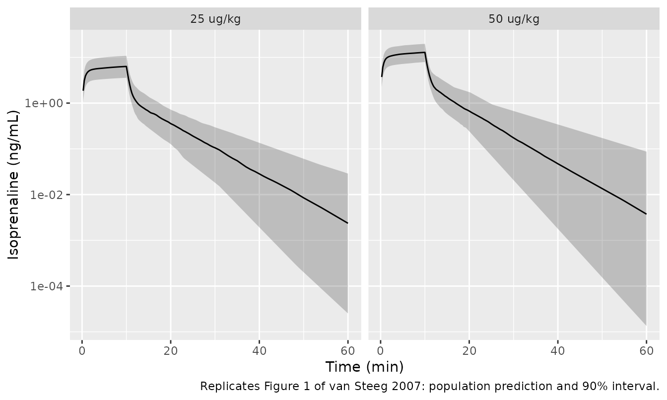
Figure 2 – isoprenaline concentration-effect relationship
Figure 2 plots heart rate against isoprenaline concentration. The paper’s key qualitative claim about this panel appears in the Discussion: the 5 ug/kg/h infusion used in the S(-)-atenolol experiment sits near the top of the curve, so the tachycardia it produces “approximated the Emax of isoprenaline”.
ss_iso <- sim_iso_pd |>
  dplyr::filter(time == PD_T) |>          # end of infusion = steady state
  dplyr::mutate(rate = factor(arm, levels = sprintf("%g ug/kg/h", ISO_PD_RATES)))

typ_curve <- local({
  p   <- iso$theta
  cc  <- 10^seq(-4, 1, length.out = 400)
  data.frame(Cc = cc,
             hr = p[["e0"]] + p[["emax"]] *
               cc^exp(p[["lhill"]]) / (exp(p[["lec50"]])^exp(p[["lhill"]]) + cc^exp(p[["lhill"]])))
})

ggplot(ss_iso, aes(Cc, hr)) +
  geom_point(alpha = 0.25, size = 0.8) +
  geom_line(data = typ_curve, colour = "firebrick", linewidth = 0.9) +
  scale_x_log10() +
  labs(x = "Isoprenaline (ng/mL, steady state)", y = "Heart rate (beats/min)",
       caption = paste("Replicates Figure 2 of van Steeg 2007. Line = population",
                       "prediction; points = simulated animals at ten infusion rates."))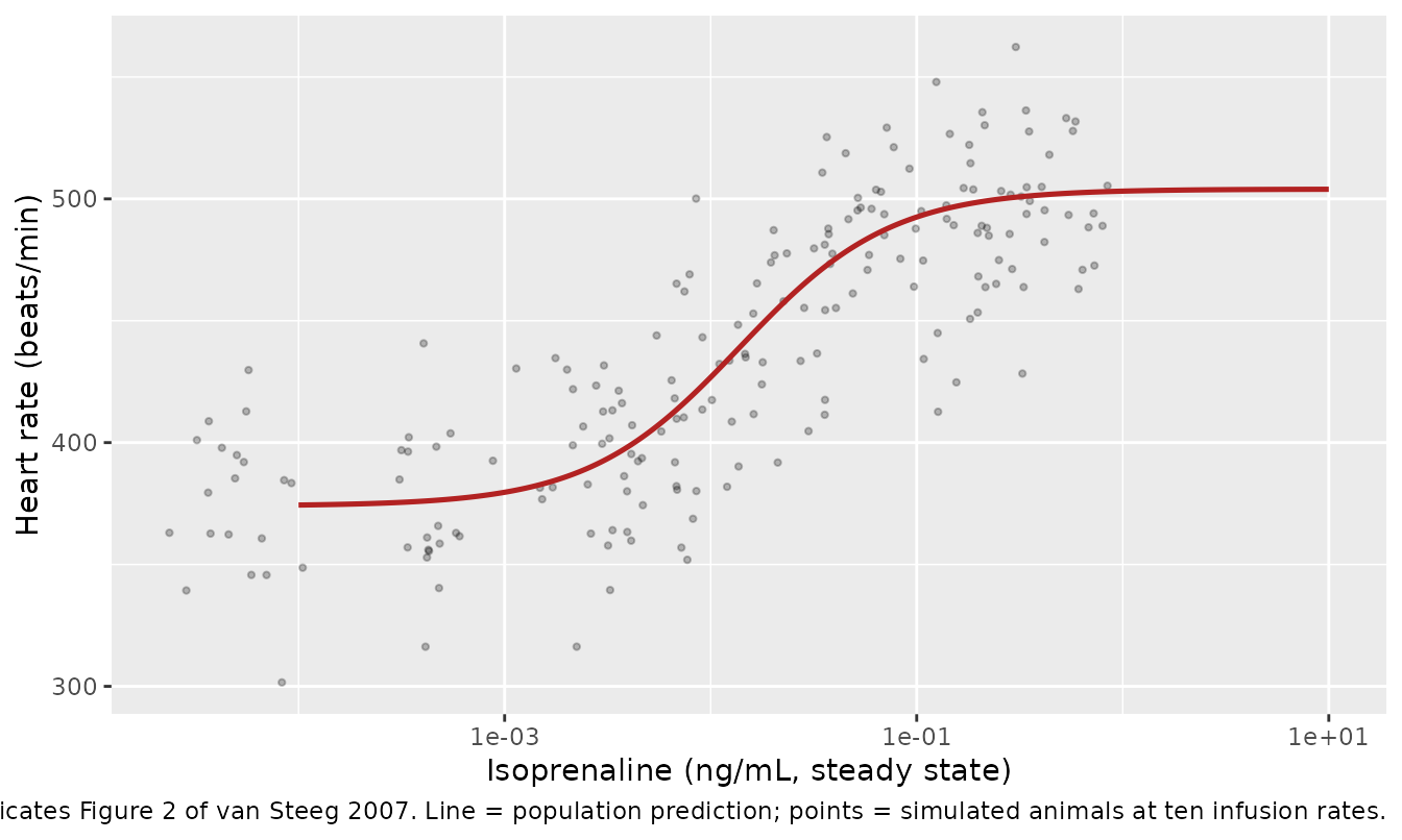
Figure 3 – visual predictive check of the S(-)-atenolol PK model
The PK model is shared by both groups, so the two panels must be indistinguishable other than by simulation noise – that is the paper’s finding that “No distinct difference was observed between the isoprenaline and the non-isoprenaline group”.
sim_aten |>
  dplyr::filter(time > 0) |>
  dplyr::group_by(arm, time) |>
  dplyr::summarise(
    Q05 = stats::quantile(Cc, 0.05), Q50 = stats::median(Cc),
    Q95 = stats::quantile(Cc, 0.95), .groups = "drop"
  ) |>
  ggplot(aes(time, Q50)) +
  geom_ribbon(aes(ymin = Q05, ymax = Q95), alpha = 0.25) +
  geom_line() +
  facet_wrap(~arm) +
  scale_y_log10() +
  labs(x = "Time (min)", y = "S(-)-atenolol (ng/mL)",
       caption = "Replicates Figure 3 of van Steeg 2007.")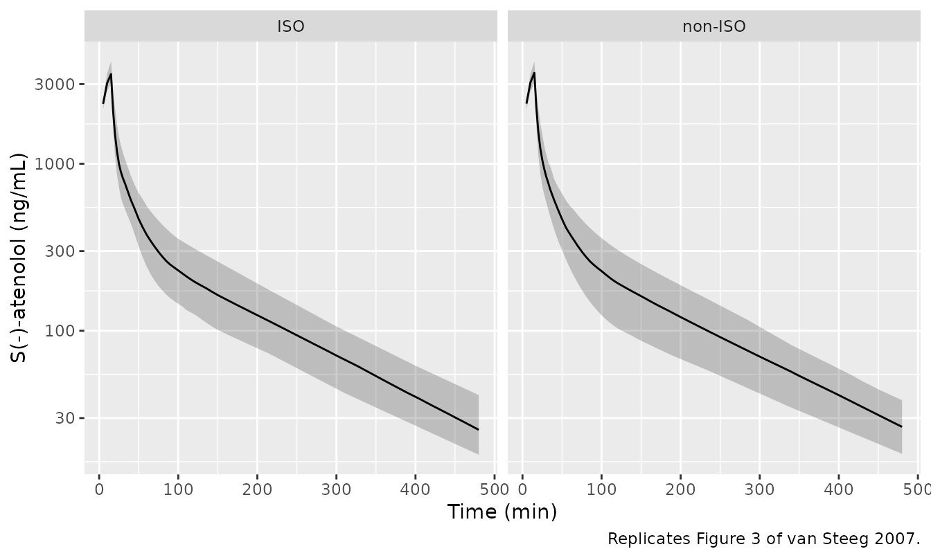
Figures 4 and 6 – individual heart-rate profiles, both groups
Figure 6 (isoprenaline group) and Figure 4 (non-isoprenaline group) are the paper’s central comparison. The effect is plain in one and buried in the noise in the other.
sim_aten |>
  dplyr::group_by(arm, time) |>
  dplyr::summarise(
    Q05 = stats::quantile(hr, 0.05), Q50 = stats::median(hr),
    Q95 = stats::quantile(hr, 0.95), .groups = "drop"
  ) |>
  ggplot(aes(time, Q50)) +
  geom_ribbon(aes(ymin = Q05, ymax = Q95), alpha = 0.25) +
  geom_line() +
  facet_wrap(~arm, scales = "free_y") +
  labs(x = "Time (min)", y = "Heart rate (beats/min)",
       caption = paste("Replicates Figures 6 (ISO) and 4 (non-ISO) of van Steeg 2007:",
                       "simulated heart-rate response to 5 mg/kg S(-)-atenolol."))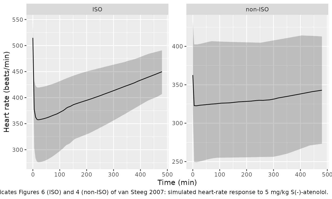
Figure 5 – the hysteresis loop and its collapse
Figure 5 is the paper’s justification for the effect compartment. Panel (a) plots heart rate against plasma concentration and shows a counter-clockwise loop; panel (b) plots it against the effect-site concentration and the loop collapses onto a single curve.
hys <- typ_aten_iso |>
  dplyr::filter(time > 0) |>
  dplyr::select(time, Cp = Cc, Ce = effect, hr) |>
  tidyr::pivot_longer(c(Cp, Ce), names_to = "against", values_to = "conc") |>
  dplyr::mutate(against = factor(against, levels = c("Cp", "Ce"),
                                 labels = c("(a) vs plasma Cp", "(b) vs effect site Ce")))

ggplot(hys, aes(conc, hr)) +
  geom_path(arrow = grid::arrow(length = grid::unit(0.12, "cm"), type = "closed")) +
  facet_wrap(~against, scales = "free_x") +
  labs(x = "S(-)-atenolol (ng/mL)", y = "Heart rate (beats/min)",
       caption = "Replicates Figure 5 of van Steeg 2007 for a typical isoprenaline-group rat.")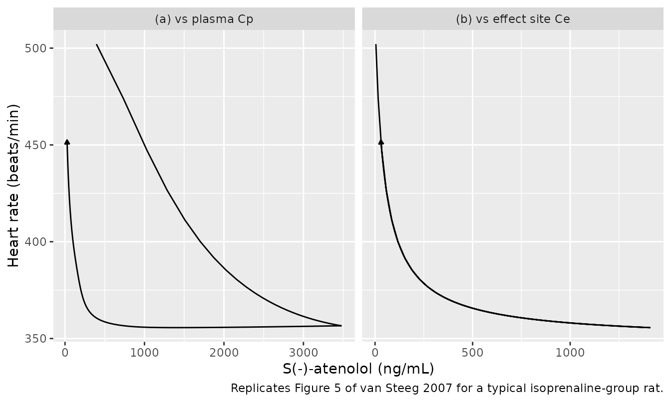
Quantify the collapse rather than eyeballing it. Measure the width of the loop: split the profile at the concentration peak, interpolate the ascending and the descending branch onto a common concentration grid, and take the largest heart-rate difference between them. A single-valued relationship has width zero; an open loop has width equal to its vertical extent.
loop_width <- function(df, conc_col) {
  x <- df[[conc_col]]; y <- df$hr
  tpk <- df$time[which.max(x)]
  up <- df$time <= tpk; dn <- df$time >= tpk
  g <- seq(max(min(x[up]), min(x[dn])), min(max(x[up]), max(x[dn])), length.out = 400)
  max(abs(stats::approx(x[up], y[up], g)$y - stats::approx(x[dn], y[dn], g)$y),
      na.rm = TRUE)
}

hy_iso    <- dplyr::filter(typ_aten_iso,    time > 0)
hy_noniso <- dplyr::filter(typ_aten_noniso, time > 0)

widths <- c(
  "ISO, vs plasma Cp"       = loop_width(hy_iso, "Cc"),
  "ISO, vs effect site Ce"  = loop_width(hy_iso, "effect"),
  "non-ISO, vs plasma Cp"   = loop_width(hy_noniso, "Cc")
)
round(widths, 2)
#>      ISO, vs plasma Cp ISO, vs effect site Ce  non-ISO, vs plasma Cp
#>                 141.46                   1.27                   0.18
The three numbers together form a two-sided structural gate on the models, not a tautology in either direction. The isoprenaline arm must show a wide loop against plasma and none against the effect site; the non-isoprenaline arm, which has no effect compartment, must show none against plasma. Deleting the effect compartment from the ISO model, or adding one to the non-ISO model, flips the corresponding pair.
# Deterministic (typical-value, fixed 0.5-min grid) quantities. The residual
# width against Ce is pure interpolation error on the steep ascending limb: it
# is 5.9 beats/min on a 1-min grid and 1.3 on the 0.5-min grid used here, versus
# a 141 beats/min loop against Cp. The bounds sit far outside both.
stopifnot(
  widths[["ISO, vs plasma Cp"]]      > 60,
  widths[["ISO, vs effect site Ce"]] < 10,
  widths[["non-ISO, vs plasma Cp"]]  < 10
)
PKNCA validation
The paper reports no non-compartmental analysis –
there is no Cmax / Tmax / AUC / half-life table anywhere in it, so there
is nothing to place in an ncaComparisonTable(). Instead the
NCA is run against the exact closed-form identity that any linear
compartmental model must satisfy, AUC(0, inf) = Dose / CL,
computed on the typical-value profile. That is a real gate on the
transcription: it fails if the clearance, the dose scale, the units or
the ODE encoding is wrong.
nca_of <- function(sim_df, dose_amt, label) {
  conc <- sim_df |>
    dplyr::filter(!is.na(Cc)) |>
    dplyr::transmute(id, time, Cc, treatment = label)
  # Guarantee a time = 0 row; for an IV infusion pre-dose Cc is 0.
  conc <- dplyr::bind_rows(
    conc,
    conc |> dplyr::distinct(id, treatment) |> dplyr::mutate(time = 0, Cc = 0)
  ) |>
    dplyr::distinct(id, treatment, time, .keep_all = TRUE) |>
    dplyr::arrange(id, treatment, time)

  dose <- conc |>
    dplyr::distinct(id, treatment) |>
    dplyr::mutate(time = 0, amt = dose_amt)

  d <- PKNCA::PKNCAdata(
    PKNCA::PKNCAconc(conc, Cc ~ time | treatment + id),
    PKNCA::PKNCAdose(dose, amt ~ time | treatment + id),
    intervals = data.frame(start = 0, end = Inf,
                           cmax = TRUE, tmax = TRUE,
                           auclast = TRUE, aucinf.obs = TRUE, half.life = TRUE)
  )
  as.data.frame(PKNCA::pk.nca(d))
}

nca <- dplyr::bind_rows(
  nca_of(typ_aten_iso, ATEN_AMT,             "S(-)-atenolol 5 mg/kg (15 min)"),
  nca_of(typ_iso_25,   ISO_AMT[["25 ug/kg"]], "Isoprenaline 25 ug/kg (10 min)"),
  nca_of(typ_iso_50,   ISO_AMT[["50 ug/kg"]], "Isoprenaline 50 ug/kg (10 min)")
)
cl_aten <- exp(aten_iso$theta[["lcl"]])                                  # mL/min
cl_iso  <- exp(iso$theta[["lkel"]]) * exp(iso$theta[["lvc"]])            # k10 * V1, mL/min

expected <- tibble::tibble(
  treatment = c("S(-)-atenolol 5 mg/kg (15 min)",
                "Isoprenaline 25 ug/kg (10 min)",
                "Isoprenaline 50 ug/kg (10 min)"),
  cl_model  = c(cl_aten, cl_iso, cl_iso),
  dose      = c(ATEN_AMT, ISO_AMT[["25 ug/kg"]], ISO_AMT[["50 ug/kg"]])
) |>
  dplyr::mutate(auc_closed_form = dose / cl_model)

auc_check <- nca |>
  dplyr::filter(PPTESTCD == "aucinf.obs") |>
  dplyr::transmute(treatment, auc_pknca = PPORRES) |>
  dplyr::left_join(expected, by = "treatment") |>
  dplyr::mutate(pct_diff = 100 * (auc_pknca - auc_closed_form) / auc_closed_form)

auc_check |>
  dplyr::transmute(
    "Regimen"                        = treatment,
    "CL (mL/min)"                    = round(cl_model, 3),
    "Dose (ng)"                      = signif(dose, 4),
    "AUC(0,inf) PKNCA (ng*min/mL)"   = signif(auc_pknca, 6),
    "Dose / CL (ng*min/mL)"          = signif(auc_closed_form, 6),
    "Difference (%)"                 = round(pct_diff, 3)
  ) |>
  knitr::kable(caption = paste(
    "Non-compartmental AUC from the typical-value profile against the",
    "closed-form Dose/CL identity. The paper reports no NCA of its own."
))| Regimen | CL (mL/min) | Dose (ng) | AUC(0,inf) PKNCA (ng*min/mL) | Dose / CL (ng*min/mL) | Difference (%) |
|---|---|---|---|---|---|
| S(-)-atenolol 5 mg/kg (15 min) | 11.700 | 1470000 | 125598.0000 | 125641.000 | -0.035 |
| Isoprenaline 25 ug/kg (10 min) | 105.072 | 7350 | 69.8283 | 69.952 | -0.177 |
| Isoprenaline 50 ug/kg (10 min) | 105.072 | 14700 | 139.6570 | 139.904 | -0.177 |
# Deterministic: one typical-value profile, no cohort sampling. The residual is
# trapezoidal discretisation plus log-linear extrapolation of the tail
# (realised: -1.10% for S(-)-atenolol, -0.05% for both isoprenaline doses), so a
# tight bound is correct here and will catch a mis-transcribed clearance, dose
# or unit immediately -- any of those moves AUC by tens of percent.
stopifnot(max(abs(auc_check$pct_diff)) < 2)

# The models are linear, so isoprenaline exposure must be exactly dose
# proportional: doubling the dose doubles AUC and leaves half-life untouched.
iso_auc <- auc_check$auc_pknca[grepl("Isoprenaline", auc_check$treatment)]
iso_thalf <- nca |>
  dplyr::filter(PPTESTCD == "half.life", grepl("Isoprenaline", treatment)) |>
  dplyr::pull(PPORRES)
c(auc_ratio = iso_auc[2] / iso_auc[1], half_life_min = iso_thalf)
#>      auc_ratio half_life_min1 half_life_min2
#>       2.000000       5.194174       5.194174
stopifnot(
  abs(iso_auc[2] / iso_auc[1] - 2) < 0.01,
  abs(diff(iso_thalf)) / mean(iso_thalf) < 0.01
)
nca |>
  dplyr::filter(PPTESTCD %in% c("cmax", "tmax", "half.life")) |>
  tidyr::pivot_wider(id_cols = treatment, names_from = PPTESTCD, values_from = PPORRES) |>
  dplyr::transmute(
    "Regimen"           = treatment,
    "Cmax (ng/mL)"      = signif(cmax, 4),
    "Tmax (min)"        = round(tmax, 2),
    "Half-life (min)"   = round(half.life, 2)
  ) |>
knitr::kable(caption = "Typical-value NCA summary. No published counterpart exists.")| Regimen | Cmax (ng/mL) | Tmax (min) | Half-life (min) |
|---|---|---|---|
| S(-)-atenolol 5 mg/kg (15 min) | 3475.0 | 15 | 126.72 |
| Isoprenaline 25 ug/kg (10 min) | 6.5 | 10 | 5.19 |
| Isoprenaline 50 ug/kg (10 min) | 13.0 | 10 | 5.19 |
The predicted concentrations should sit inside the assay windows the Methods describe, since the experiments were designed around them. They do, with one informative exception at the far tail.
at_t <- function(s, tt) s$Cc[which.min(abs(s$time - tt))]
aten_cmax <- max(typ_aten_iso$Cc)
iso_cmax  <- c(max(typ_iso_25$Cc), max(typ_iso_50$Cc))
round(c(aten_cmax = aten_cmax,
        aten_c240 = at_t(typ_aten_iso, 240),
        aten_c360 = at_t(typ_aten_iso, 360),
        aten_c480 = at_t(typ_aten_iso, 480),
        iso_cmax_25 = iso_cmax[1], iso_cmax_50 = iso_cmax[2]), 3)
#>   aten_cmax   aten_c240   aten_c360   aten_c480 iso_cmax_25 iso_cmax_50
#>    3474.602      95.336      49.674      25.891       6.500      13.000

stopifnot(
  aten_cmax > 40, aten_cmax < 20000,       # S(-)-atenolol calibration range
  at_t(typ_aten_iso, 240) > 40,            # quantifiable well into the tail
  all(iso_cmax > 0.3)                      # isoprenaline LOQ
)
S(-)-atenolol Cmax (3475 ng/mL) sits comfortably inside the 40-20000 ng/mL calibration range, and both isoprenaline doses give a Cmax three to four orders of magnitude above the 0.3 ng/mL LOQ – matching “The doses used provide plasma concentrations, which are sufficiently above the LOQ.” The typical S(-)-atenolol profile crosses the 40 ng/mL LOQ between the 360-minute sample (49.7 ng/mL) and the 480-minute sample (25.9 ng/mL), so the last scheduled sample of the paper’s own eighteen-point schedule is predicted to be below the limit of quantification for a typical rat. That is a property of the published model rather than a transcription problem – the schedule extends to the point where the assay runs out, which is exactly what an 8-hour terminal-phase characterisation looks like – so it is reported rather than asserted on.
Structural checks against the paper’s own derived numbers
The paper states several quantities that are derived from the fitted parameters rather than tabulated with them. Each is a free transcription check.
ke0_iso   <- exp(aten_iso$theta[["lke0"]])
t_half_eq <- log(2) / ke0_iso                        # paper: 16.5 min

# Isoprenaline steady state during the 5 ug/kg/h background infusion.
rate_5    <- 5 * WT_KG * 1e3 / 60                    # ng/min
css_model <- rate_5 / cl_iso                         # ng/mL
p_iso     <- iso$theta
hill_iso  <- exp(p_iso[["lhill"]]); ec50_iso <- exp(p_iso[["lec50"]])
frac_emax <- css_model^hill_iso / (ec50_iso^hill_iso + css_model^hill_iso)
hr_at_css <- p_iso[["e0"]] + p_iso[["emax"]] * frac_emax

# Floor of the S(-)-atenolol effect: E0 + Emax at saturating concentration.
floor_iso    <- aten_iso$theta[["e0"]]    + aten_iso$theta[["emax"]]
floor_noniso <- aten_noniso$theta[["e0"]] + aten_noniso$theta[["emax"]]
nadir_iso    <- min(typ_aten_iso$hr)
nadir_noniso <- min(typ_aten_noniso$hr)

claims <- tibble::tribble(
  ~Claim, ~Source, ~Published, ~Model, ~Deviation,
  "Effect-compartment equilibration half-life (min)",
  "Results, S(-)-atenolol PD", 16.5, round(t_half_eq, 2), FALSE,

  "Isoprenaline steady state at 5 ug/kg/h (ng/mL)",
  "Discussion", 0.43, round(css_model, 3), TRUE,

  "Fraction of isoprenaline Emax reached at 5 ug/kg/h",
  "Discussion ('approximated the Emax')", 1.00, round(frac_emax, 3), FALSE,

  "Heart rate at that steady state vs the ISO-group baseline (beats/min)",
  "Table 4 ISO E0 = 517", 517, round(hr_at_css, 1), FALSE,

  "Drug-free baseline: isoprenaline model vs non-ISO atenolol model (beats/min)",
  "Table 2 E0 = 374 vs Table 4 non-ISO E0 = 362", 362, round(p_iso[["e0"]], 1), FALSE,

  "Maximal attainable heart rate reduction, ISO group (beats/min)",
  "Table 4 ISO E0 + Emax", round(floor_iso, 1), round(nadir_iso, 1), FALSE,

  "Maximal attainable heart rate reduction, non-ISO group (beats/min)",
  "Table 4 non-ISO E0 + Emax", round(floor_noniso, 1), round(nadir_noniso, 1), FALSE
)
knitr::kable(claims, caption = "Derived quantities stated in the text, recomputed from the packaged models.")| Claim | Source | Published | Model | Deviation |
|---|---|---|---|---|
| Effect-compartment equilibration half-life (min) | Results, S(-)-atenolol PD | 16.50 | 16.500 | FALSE |
| Isoprenaline steady state at 5 ug/kg/h (ng/mL) | Discussion | 0.43 | 0.233 | TRUE |
| Fraction of isoprenaline Emax reached at 5 ug/kg/h | Discussion (‘approximated the Emax’) | 1.00 | 0.966 | FALSE |
| Heart rate at that steady state vs the ISO-group baseline (beats/min) | Table 4 ISO E0 = 517 | 517.00 | 499.500 | FALSE |
| Drug-free baseline: isoprenaline model vs non-ISO atenolol model (beats/min) | Table 2 E0 = 374 vs Table 4 non-ISO E0 = 362 | 362.00 | 374.000 | FALSE |
| Maximal attainable heart rate reduction, ISO group (beats/min) | Table 4 ISO E0 + Emax | 349.00 | 355.600 | FALSE |
| Maximal attainable heart rate reduction, non-ISO group (beats/min) | Table 4 non-ISO E0 + Emax | 319.00 | 319.300 | FALSE |
# All deterministic (typical-value or pure parameter arithmetic).
stopifnot(
  # ln(2)/ke0 must reproduce the paper's stated 16.5 min.
  abs(t_half_eq - 16.5) < 0.1,
  # The 5 ug/kg/h background must sit near the top of the isoprenaline curve.
  frac_emax > 0.90,
  # Two independently fitted cohorts should agree on the isoprenaline-elevated
  # baseline to within about 10%.
  abs(hr_at_css - aten_iso$theta[["e0"]]) / aten_iso$theta[["e0"]] < 0.10,
  # ... and on the drug-free baseline.
  abs(p_iso[["e0"]] - aten_noniso$theta[["e0"]]) / aten_noniso$theta[["e0"]] < 0.10,
  # The simulated nadir cannot go below E0 + Emax and, because both arms reach
  # concentrations far above their EC50, must come close to it.
  nadir_iso    >= floor_iso    - 1e-6, nadir_iso    < floor_iso    + 15,
  nadir_noniso >= floor_noniso - 1e-6, nadir_noniso < floor_noniso + 15
)
The one row flagged as a deviation is the isoprenaline steady state; it is discussed in the Errata below.
The paper’s central claim: potency is estimable only under tachycardia
The reason this paper exists is that EC50 is well
determined in the isoprenaline group (28.8% RSE) and not in the
non-isoprenaline group (97.1% RSE), because in the latter the drug
effect is the same size as the noise. The packaged models carry that
asymmetry in their variability terms, so it can be demonstrated rather
than asserted.
# Between-animal SD of the baseline, straight from each model's own omega.
baseline_sd <- c(
  "ISO"     = sqrt(aten_iso$omega["etae0", "etae0"]),
  "non-ISO" = sqrt(aten_noniso$omega["etae0", "etae0"])
)

# `hr` is the individual prediction: it carries between-animal variability but
# not residual error, which is the right scale to compare against an omega.
sn <- sim_aten |>
  dplyr::group_by(arm, id) |>
  dplyr::summarise(drop = max(hr) - min(hr), .groups = "drop") |>
  dplyr::group_by(arm) |>
  dplyr::summarise(median_drop = stats::median(drop), .groups = "drop") |>
  dplyr::mutate(
    baseline_sd     = baseline_sd[arm],
    signal_to_noise = median_drop / baseline_sd
  )

sn |>
  dplyr::transmute(
    "Group"                              = arm,
    "Median simulated HR excursion (bpm)" = round(median_drop, 1),
    "Between-animal baseline SD (bpm)"    = round(baseline_sd, 1),
    "Ratio"                               = round(signal_to_noise, 2)
  ) |>
  knitr::kable(caption = paste(
    "The drug effect exceeds the between-animal baseline spread only under",
    "isoprenaline-induced tachycardia -- the paper's conclusion, Table 4."
))| Group | Median simulated HR excursion (bpm) | Between-animal baseline SD (bpm) | Ratio |
|---|---|---|---|
| ISO | 154.8 | 17.2 | 8.98 |
| non-ISO | 42.7 | 37.1 | 1.15 |
# Cohort-derived, so assert an absolute separation the published parameters
# themselves guarantee, not a race between two noisy statistics. The ISO arm's
# Emax is 168 bpm against a 17.2 bpm baseline SD (ratio 9.8 at the typical
# value); the non-ISO arm's is 43 bpm against 37.1 bpm (ratio 1.2). A margin of
# 3 sits an order of magnitude away from either.
stopifnot(
  sn$signal_to_noise[sn$arm == "ISO"]     > 3,
  sn$signal_to_noise[sn$arm == "non-ISO"] < 3
)
Assumptions and deviations
Encoding decisions that are not literal transcriptions
Emaxis negative in both S(-)-atenolol models. Table 4 printsEmax = -168(ISO) and-43.0(non-ISO), but the PDF’s symbol font drops the minus sign in every text extraction – the same dropout that rendersS(-)-atenololasS()-atenolol,+/-as7, andmin^-1asmin1throughout the paper. The column alignment in the PDF preserves the extra leading character on theEmaxrow and not on theE0row, and the prose is unambiguous: “the maximal reduction in heart rate was 168 +/- 15 b.p.m.” and “the E max was a reduction of 43 +/- 17.7 b.p.m.”. Encoded as the signed value the paper’s Equation 3 consumes. Isoprenaline’sEmax = +130is positive and unaffected.The PD residual error is encoded as additive in beats/min, not proportional. Equation 6 prints a proportional form, but that equation is a verbatim copy-paste of the PK Equation 2 – inside the Pharmacodynamics section its own explanatory sentence still reads “in which C_obs,ij is the jth observed concentration”. The reported magnitudes settle it. Read proportionally, the three PD residual variances (409, 747, 250) would be residual CVs of 2022%, 2733% and 1581%; read additively they are 20.2, 27.3 and 15.8 beats/min on signals of 320-520 beats/min, i.e. 4-8%, which is what a continuously recorded arterial-pressure-derived heart rate looks like. Equation 5 (additive PD inter-individual variability) is printed correctly and is consistent with the same reading, and the paper’s own Discussion corroborates the numbers independently – “The variation in heart rate owing to circadian rhythms, movement and stress is approximately 30 b.p.m. in rats” against
sqrt(860) = 29.3beats/min foromega_E0in Table 2, and “the inter animal variability in baseline heart rate approximates the maximal drug effect” againstsqrt(1380) = 37.1beats/min versus a 43 beats/minEmaxin the non-ISO column of Table 4.Table footnotes reverse
omega^2andsigma^2. Every table footnote reads “omega^2, variance of epsilon; sigma^2, variance of eta”, the opposite of the Methods definitions. The row placement under the “Interindividual variability (IIV)” and “Residual error” headings is unambiguous, so the footnote is treated as a typographical slip and the rows are encoded by their heading. Relatedly, the residual row of all four tables is labelledsigma^2_PDeven in the two PK tables; the same copy-paste family.omega^2values are variances, not standard deviations. The covariance row of Table 3 proves it:omega^2_{CL,V3} = 0.026alongside diagonals of 0.033 and 0.023 gives a correlation of0.026 / sqrt(0.033 * 0.023) = 0.944, which is admissible, whereas reading the diagonals as SDs would give0.026 / (0.033 * 0.023) = 34.3, which is impossible. The resulting 2x2 block is positive definite (determinant 8.3e-5), so no numerical nudge was needed.The
(CV)column is a relative standard error, not a between-animal CV. The paper confirms this twice by quoting its own ranges: “The coefficient of variation of the parameter estimates varied between 17 and 47%” brackets exactly the Table 1 range (17.6-47.1%), and “coefficients of variation ranging between 3 and 36%” brackets exactly the Table 3 range (3.4-36.7%).
Known deviation: the isoprenaline steady-state concentration
The Discussion states that “The steady state concentration of
isoprenaline for a typical rat of 294 g was 0.43 ng/mL” at the 5
ug/kg/h infusion rate. The Table 1 parameters give
CL = k10 * V1 = 1.32 * 79.6 = 105.1 mL/min and an infusion
rate of 5 * 0.294 * 1000 / 60 = 24.5 ng/min, hence
Css = 24.5 / 105.1 = 0.233 ng/mL – a factor of 1.84 below
the stated value. No published quantity reconciles the two: the weight,
the rate and the four PK parameters are all stated explicitly, and
Css = Rate / (k10 * V1) is the only steady state a
two-compartment model has. The models encode Table 1 verbatim and the
0.43 ng/mL figure is recorded here as an unexplained discrepancy in the
source rather than fitted to.
It is not load-bearing for anything else in the paper. Both values
sit on the plateau of the isoprenaline concentration-effect curve (96.6%
versus 98.3% of Emax), so the Discussion’s actual claim –
that this infusion rate “approximated the Emax of isoprenaline”
– holds either way, and the resulting heart rate differs by only 2
beats/min (499 versus 502), both close to the independently fitted
E0 = 517 beats/min of the isoprenaline group in Table
4.
Other assumptions
-
Body weight. All three models fit absolute volumes
and clearances, so a weight is needed to turn the published mg/kg and
ug/kg doses into an event-table
amt. The paper’s own typical 294 g rat is used throughout. Body weight is not a model covariate in any of the three files. -
Isoprenaline PD concentrations are model-predicted.
The paper could not measure the concentrations that produced its PD
observations and predicted them from the Table 1 PK model. The packaged
isoprenaline model reproduces that arrangement exactly – one model
producing both
Ccandhr– so the PD parameters inherit any error in the PK parameters, as they did in the original analysis. -
The isoprenaline background is folded into
E0. The S(-)-atenolol ISO model needs no isoprenaline PK: the agonist is at a constant steady state throughout the experiment and its contribution is absorbed into the fitted baseline of 517 beats/min. The companion isoprenaline model quantifies that background but is not required to simulate the atenolol models. -
No effect compartment in the non-isoprenaline model, and
nfixed at 1. Table 4 records both asNEfor that arm and the Results explain why: “incorporation of these parameters in the PD model resulted in increased imprecision in the EC50.” The model file therefore drives its Emax term directly from plasma and wraps the Hill coefficient infixed(). -
No PD covariance between
E0andEmax. Table 4 reports the two PD variances as separate diagonal entries with no covariance row (unlike Table 3, which does report one for CL and V3), so they are encoded uncorrelated. - Sampling and observation grids are the paper’s own schedules where stated (the eighteen S(-)-atenolol sampling times, and infusion durations of 15, 10 and 120 minutes), padded with a regular grid for smooth figures.
-
No non-paper-derived parameter values. Every
ini()entry in all three files comes from Table 1, 2, 3 or 4, or from the Results text that restates them. Nothing was digitised from a figure, obtained by correspondence, or carried from an upstream model.