Model and source
- Citation: Ohk B, Seong S, Lee J, Gwon M, Kang W, Lee H, Yoon Y, Yoo H. Evaluation of sex differences in the pharmacokinetics of oral sumatriptan in healthy Korean subjects using population pharmacokinetic modeling. Biopharm Drug Dispos. 2022;43(1):24-31. doi:10.1002/bdd.2307.
- Description: One-compartment population PK model for oral sumatriptan in healthy Korean adults (Ohk 2022): two parallel absorption routes (first-order absorption with lag time, and a transit-compartment chain with the Savic 2007 analytical input form) into a single central compartment with linear elimination, with separate typical apparent clearances for males and females.
- Article: https://doi.org/10.1002/bdd.2307 (open access; PMC9306698)
Ohk 2022 re-fits the sumatriptan model of Lee 2015 (packaged as
Lee_2015_sumatriptan) to a pooled cohort that adds a second
study with female subjects, and finds that apparent oral clearance
differs by sex.
Population
Thirty-eight healthy Korean adults (29 males, 76.3%; 9 females, 23.7%) from two single-dose studies run under the same protocol at Kyungpook National University Hospital, Daegu: the male cohort of Lee 2015 and an additional study (CRIS KCT0001784) run to evaluate sex differences. Age was 24.8 +/- 2.7 years (21-31), weight 64.0 +/- 9.8 kg (50-84), height 171.1 +/- 7.8 cm, BMI 21.8 +/- 2.2 kg/m^2 and Cockcroft-Gault creatinine clearance 119.2 +/- 17.9 mL/min (Table 1, Section 3.1). Each subject received a single 50 mg sumatriptan tablet under fasting conditions; plasma was sampled pre-dose and at 0.25, 0.5, 0.75, 1, 1.5, 2, 2.5, 3, 4, 6, 8, 10 and 12 h (Section 2.2), giving 532 concentrations for the population analysis.
str(rxode2::rxode(readModelDb("Ohk_2022_sumatriptan"))$population)
#> ℹ parameter labels from comments will be replaced by 'label()'
#> List of 13
#>  $ species       : chr "human"
#>  $ n_subjects    : int 38
#>  $ n_studies     : int 2
#>  $ age_range     : chr "21-31 years"
#>  $ age_median    : chr "24.8 years (mean)"
#>  $ weight_range  : chr "50-84 kg"
#>  $ weight_median : chr "64.0 kg (mean)"
#>  $ sex_female_pct: num 23.7
#>  $ race_ethnicity: chr "Korean"
#>  $ disease_state : chr "Healthy adult volunteers"
#>  $ dose_range    : chr "Single 50 mg oral dose of sumatriptan (Sumatran 50 mg tablet) under fasting conditions"
#>  $ regions       : chr "Republic of Korea (Kyungpook National University Hospital Clinical Trial Center, Daegu)"
#>  $ notes         : chr "Pooled analysis of two single-dose studies run with the same protocol: the male cohort previously analysed by L"| __truncated__
Source trace
| Equation / parameter | Value | Source location |
|---|---|---|
lcl_male (CL/F, males) |
log(444) | Table 4 CL/F M = 444 L/h (RSE 4%); also Section 3.4 |
lcl_female (CL/F, females) |
log(281) | Table 4 CL/F F = 281 L/h (RSE 7%); also Section 3.4 |
lvc (V/F) |
log(68.7) | Table 4 V3/F = 68.7 L (RSE 32%) |
lka1 (first-order absorption rate) |
log(0.568) | Table 4 ka1 = 0.568 1/h (RSE 12%) |
lka2 (final transit compartment -> central) |
log(0.295) | Table 4 ka2 = 0.295 1/h (RSE 5%) |
lmtt (mean transit time) |
log(1.52) | Table 4 MTT = 1.52 h (RSE 11%) |
lntr (number of transit compartments) |
log(6.7) | Table 4 NN = 6.7 (RSE 48%) |
ltlag (lag time of the first-order arm) |
log(0.239) | Table 4 ALAG1 = 0.239 h (RSE 1%) |
lfr (fraction through the transit arm) |
log(0.558) | Table 4 f = 0.558 (RSE 7%) |
etalcl |
0.03016 | Table 4 BSV CL/F = 17.5 CV%; log(1 + 0.175^2) |
etalvc |
0.69215 | Table 4 BSV V3/F = 99.9 CV%; log(1 + 0.999^2) |
etalka2 |
0.05172 | Table 4 BSV ka2 = 23.04 CV%; log(1 + 0.2304^2) |
etalmtt |
0.16554 | Table 4 BSV MTT = 42.43 CV%; log(1 + 0.4243^2) |
propSd |
0.249 | Table 4 proportional error = 0.249 (RSE 6%) |
addSd (ng/mL) |
0.276 | Table 4 additive error = 0.276 (RSE 21%) |
| CL/F = ((1 - SEX) theta_male + SEX theta_female) exp(eta) | n/a | Table 3 model 4; SEX coded 0 = male, 1 = female (Section 2.5) |
| One compartment, parallel first-order (lag) and transit absorption | n/a | Section 2.4, Section 3.3 and Figure 1 |
| ktr = (n + 1) / MTT; a_n(t) = f Dose (ktr t)^n / n! exp(-ktr t) | n/a | Section 2.4 equations; implemented with rxode2
transit(ntr, mtt, fr)
|
| Combined proportional and additive residual error | n/a | Section 2.4 |
Virtual cohort
Individual data are not public. The virtual cohort below has 200 males and 200 females (sex is the only covariate in the final model), each given a single 50 mg oral dose and sampled on the study grid.
The model has two parallel absorption arms, so each administration
carries two dose records with the same amount: one to
depot (first-order arm, scaled by
f(depot) = 1 - fr) and one to depot2 (transit
arm; the bolus is suppressed by f(depot2) = 0 and the drug
enters through transit()).
obs_grid <- c(0, 0.25, 0.5, 0.75, 1, 1.5, 2, 2.5, 3, 4, 6, 8, 10, 12)
n_per_sex <- 200L

make_events <- function(ids, sexf, times) {
  one_id <- function(id) {
    rbind(
      data.frame(id = id, time = 0, evid = 1L, amt = 50, cmt = "depot"),
      data.frame(id = id, time = 0, evid = 1L, amt = 50, cmt = "depot2"),
      data.frame(id = id, time = times, evid = 0L, amt = 0, cmt = "central")
    )
  }
  ev <- do.call(rbind, lapply(ids, one_id))
  ev$SEXF <- sexf[match(ev$id, ids)]
  ev
}

ids <- seq_len(2L * n_per_sex)
sexf <- rep(c(0L, 1L), each = n_per_sex)
events <- make_events(ids, sexf, obs_grid)
events$sex <- ifelse(events$SEXF == 1L, "Female", "Male")
Simulation
mod <- readModelDb("Ohk_2022_sumatriptan")
rxode2::rxSetSeed(20222307)
sim <- as.data.frame(rxode2::rxSolve(mod, events = events, keep = c("sex")))
#> ℹ parameter labels from comments will be replaced by 'label()'
Typical-value checks
With linear elimination and a dose split whose fractions sum to one,
the typical-value AUC from 0 to infinity must equal Dose / (CL/F) in
each sex: 50 mg / 444 L/h = 112.6 ng.h/mL for males and 50 mg / 281 L/h
= 177.9 ng.h/mL for females. Integrating the typical profile to 72 h
checks both the transit() input scaling (the arm with
fraction fr) and the sex covariate in one step.
typ_grid <- c(seq(0, 12, by = 0.02), seq(12.5, 72, by = 0.5))
typ_events <- make_events(1:2, c(0L, 1L), typ_grid)
typ <- as.data.frame(rxode2::rxSolve(rxode2::zeroRe(mod), events = typ_events))
#> ℹ parameter labels from comments will be replaced by 'label()'
#> ℹ omega/sigma items treated as zero: 'etalcl', 'etalvc', 'etalka2', 'etalmtt'
#> Warning: multi-subject simulation without without 'omega'
typ$sex <- ifelse(typ$id == 2, "Female", "Male")

trap <- function(x, y) sum(diff(x) * (head(y, -1) + tail(y, -1)) / 2)
typ_auc <- typ |>
  dplyr::group_by(sex) |>
  dplyr::summarise(
    auc_numeric = trap(time, Cc),
    cmax = max(Cc),
    tmax = time[which.max(Cc)],
    .groups = "drop"
  ) |>
  dplyr::mutate(auc_closed_form = 50 * 1000 / ifelse(sex == "Male", 444, 281))
knitr::kable(typ_auc, digits = 2,
caption = "Typical-value AUC0-72 (trapezoidal, 0.02 h grid) vs Dose / (CL/F).")| sex | auc_numeric | cmax | tmax | auc_closed_form |
|---|---|---|---|---|
| Female | 177.94 | 36.22 | 2.00 | 177.94 |
| Male | 112.61 | 23.05 | 1.94 | 112.61 |
# Same parameters on both sides: the only difference is quadrature error
# and the < 0.1% of AUC beyond 72 h.
stopifnot(all(abs(typ_auc$auc_numeric / typ_auc$auc_closed_form - 1) < 0.01))

ggplot(typ |> dplyr::filter(time <= 12), aes(time, Cc, colour = sex)) +
  geom_line(linewidth = 0.8) +
  scale_x_continuous(breaks = c(0, 1, 2, 3, 4, 6, 8, 10, 12)) +
  labs(x = "Time after dose (h)", y = "Sumatriptan plasma conc (ng/mL)",
       colour = NULL,
       title = "Typical-value profiles after a single 50 mg oral dose") +
  theme_minimal()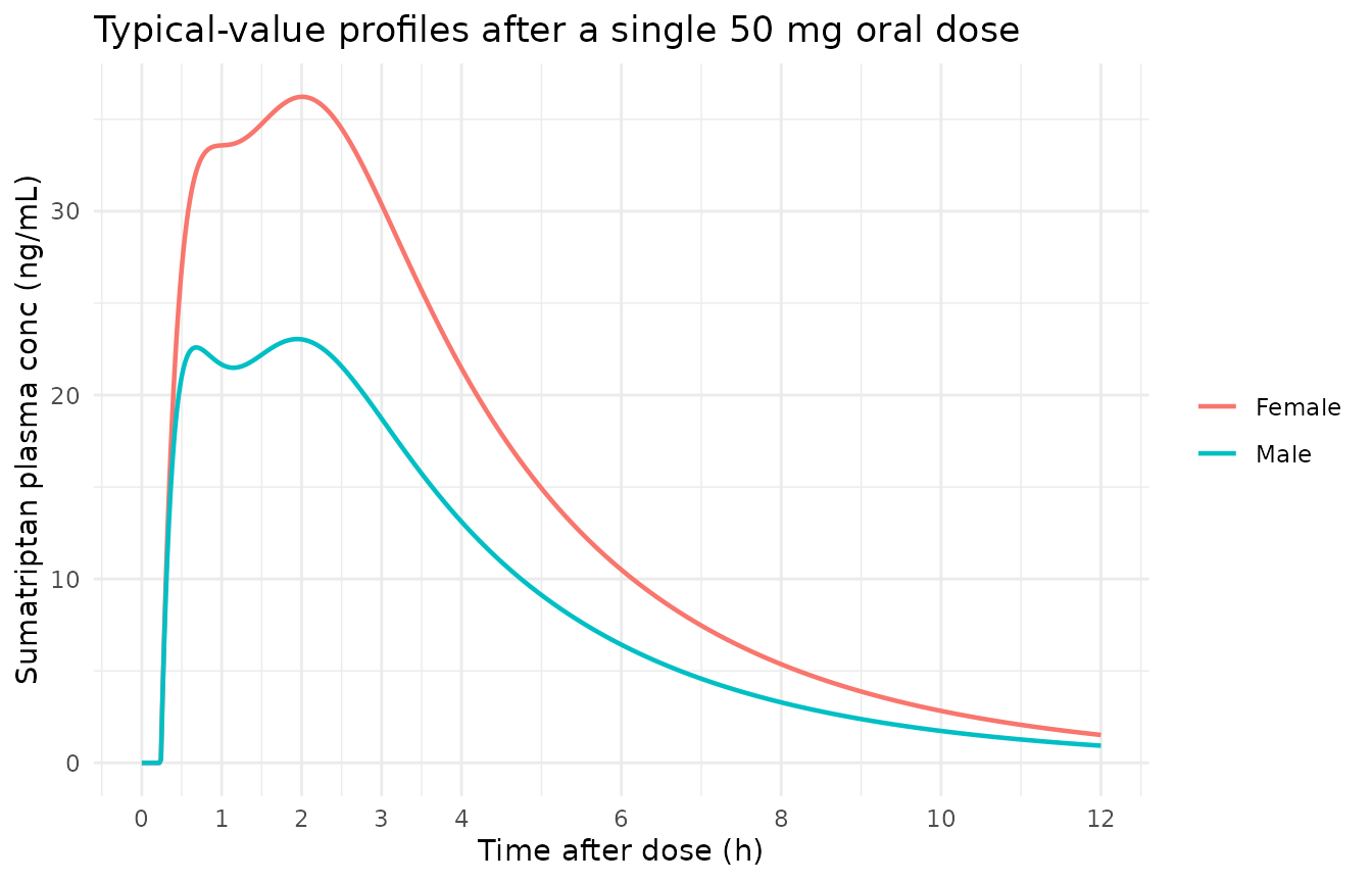
The typical profile shows the early lagged first-order peak and the later transit-arm shoulder that produce the multiple peaks described in Section 3.2.
Replicate published figures
Figure 2 – individual profiles with the median by sex
med <- sim |>
  dplyr::group_by(sex, time) |>
  dplyr::summarise(Cc = median(Cc), .groups = "drop")

ggplot(sim, aes(time, Cc)) +
  geom_line(aes(group = id), alpha = 0.08, colour = "gray40") +
  geom_line(data = med, aes(colour = sex), linewidth = 1.1) +
  scale_x_continuous(breaks = c(0, 1, 2, 3, 4, 6, 8, 10, 12)) +
  labs(x = "Time after dose (h)", y = "Sumatriptan plasma conc (ng/mL)",
       colour = "Median",
       title = "Simulated individual profiles (200 per sex)",
       subtitle = "Replicates Ohk 2022 Figure 2") +
  theme_minimal()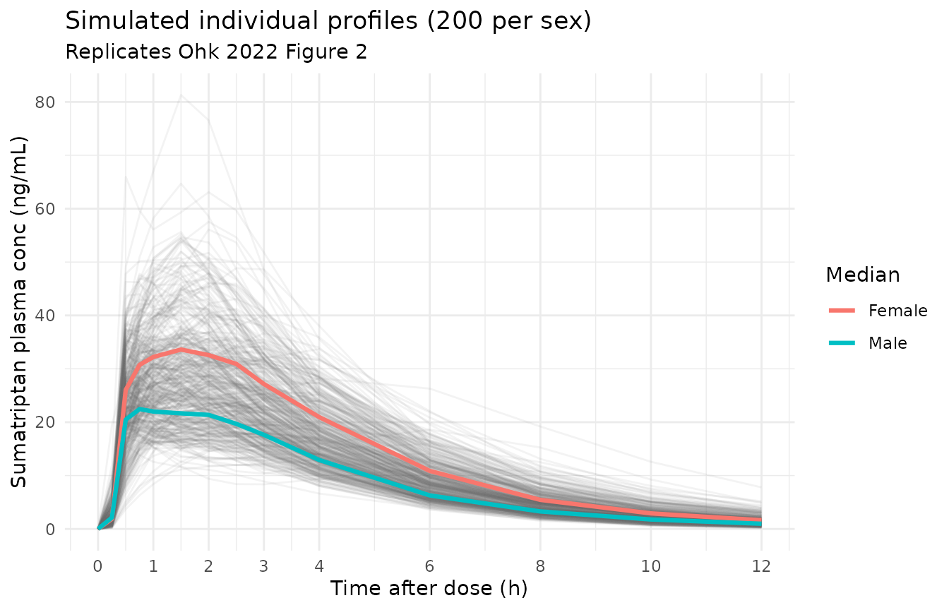
Figure 4 – individual CL/F by sex
cl_ind <- sim |>
  dplyr::filter(time == 0) |>
  dplyr::distinct(id, sex, cl)

ggplot(cl_ind, aes(sex, cl)) +
  geom_boxplot() +
  labs(x = NULL, y = "CL/F (L/h)",
       title = "Simulated individual apparent clearance by sex",
       subtitle = "Replicates Ohk 2022 Figure 4") +
  theme_minimal()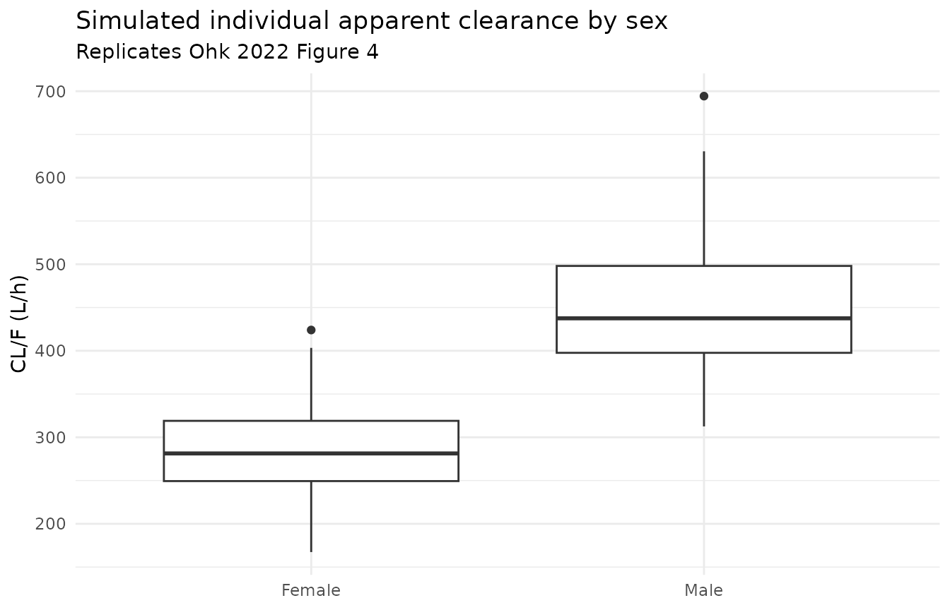
Figure 5 – visual predictive check by sex
vpc <- sim |>
  dplyr::group_by(sex, time) |>
  dplyr::summarise(
    p05 = quantile(Cc, 0.05),
    p50 = quantile(Cc, 0.50),
    p95 = quantile(Cc, 0.95),
    .groups = "drop"
  )

ggplot(vpc, aes(time, p50)) +
  geom_ribbon(aes(ymin = p05, ymax = p95), fill = "gray75") +
  geom_line(linewidth = 0.8) +
  facet_wrap(~sex) +
  scale_x_continuous(breaks = c(0, 2, 4, 6, 8, 10, 12)) +
  labs(x = "Time after dose (h)", y = "Sumatriptan plasma conc (ng/mL)",
       title = "Simulated 5th, 50th and 95th percentiles",
       subtitle = "Replicates Ohk 2022 Figure 5 (males left, females right)") +
  theme_minimal()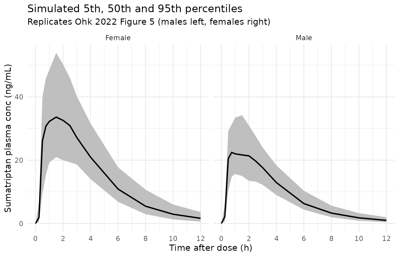
PKNCA validation
conc_df <- sim |>
  dplyr::filter(!is.na(Cc)) |>
  dplyr::select(id, time, Cc, sex)
dose_df <- events |>
  dplyr::filter(evid == 1, cmt == "depot") |>
  dplyr::select(id, time, amt, sex)

conc_obj <- PKNCA::PKNCAconc(conc_df, Cc ~ time | sex + id,
                             concu = "ng/mL", timeu = "h")
dose_obj <- PKNCA::PKNCAdose(dose_df, amt ~ time | sex + id, doseu = "mg")

intervals <- data.frame(
  start = c(0, 0),
  end = c(Inf, 2),
  cmax = c(TRUE, FALSE),
  tmax = c(TRUE, FALSE),
  auclast = c(TRUE, FALSE),
  aucinf.obs = c(TRUE, FALSE),
  half.life = c(TRUE, FALSE),
  aucint.last = c(FALSE, TRUE)
)

nca_res <- PKNCA::pk.nca(PKNCA::PKNCAdata(conc_obj, dose_obj, intervals = intervals))
nca_ind <- as.data.frame(nca_res$result)
Comparison against published NCA
Table 2 of Ohk 2022 reports geometric means for AUC and Cmax, the
median for Tmax and the arithmetic mean for t1/2. The simulated values
are summarised with the same statistics before comparison.
aucint.last is AUC0-2 and auclast is AUC0-12
(the last sample is at 12 h).
gm <- function(x) exp(mean(log(x[x > 0])))
sim_summary <- nca_ind |>
  dplyr::filter(PPTESTCD %in% c("cmax", "tmax", "auclast", "aucinf.obs",
                                "half.life", "aucint.last")) |>
  dplyr::group_by(sex, PPTESTCD) |>
  dplyr::summarise(
    value = dplyr::case_when(
      dplyr::first(PPTESTCD) == "tmax" ~ median(PPORRES, na.rm = TRUE),
      dplyr::first(PPTESTCD) == "half.life" ~ mean(PPORRES, na.rm = TRUE),
      TRUE ~ gm(PPORRES)
    ),
    .groups = "drop"
  ) |>
  tidyr::pivot_wider(names_from = PPTESTCD, values_from = value)

published <- tibble::tribble(
  ~sex,     ~aucint.last, ~auclast, ~aucinf.obs, ~cmax, ~tmax, ~half.life,
  "Male",   34.7,         111.3,    117.1,       29.0,  1.5,   2.9,
  "Female", 52.9,         182.0,    188.9,       41.4,  1.5,   2.6
)

cmp <- nlmixr2lib::ncaComparisonTable(
  simulated = sim_summary,
  reference = published,
  by = "sex",
  units = c(cmax = "ng/mL", tmax = "h", auclast = "ng*h/mL",
            aucinf.obs = "ng*h/mL", aucint.last = "ng*h/mL", half.life = "h"),
  tolerance_pct = 20
)
#> Warning: ncaParamLabel(): unknown PKNCA code(s) returned as-is: 'aucint.last'
cmp[[1]] <- sub("^aucint\\.last.*$", "AUC0-2 (ng*h/mL)", cmp[[1]])
knitr::kable(cmp, caption = "Simulated vs. published (Ohk 2022 Table 2) NCA. * differs from reference by >20%.")| NCA parameter | sex | Reference | Simulated | % diff |
|---|---|---|---|---|
| Cmax (ng/mL) | Male | 29 | 24.4 | -15.8% |
| Cmax (ng/mL) | Female | 41.4 | 36.8 | -11.2% |
| Tmax (h) | Male | 1.5 | 1 | -33.3%* |
| Tmax (h) | Female | 1.5 | 1.5 | +0.0% |
| AUC0-∞ (obs) (ng*h/mL) | Male | 117 | 111 | -4.9% |
| AUC0-∞ (obs) (ng*h/mL) | Female | 189 | 176 | -6.9% |
| AUClast (ng*h/mL) | Male | 111 | 108 | -3.3% |
| AUClast (ng*h/mL) | Female | 182 | 170 | -6.8% |
| t½ (h) | Male | 2.9 | 2.28 | -21.4%* |
| t½ (h) | Female | 2.6 | 2.24 | -13.8% |
| AUC0-2 (ng*h/mL) | Male | 34.7 | 35.7 | +3.0% |
| AUC0-2 (ng*h/mL) | Female | 52.9 | 51.5 | -2.7% |
auc_ratio <- sim_summary$aucinf.obs[sim_summary$sex == "Female"] /
  sim_summary$aucinf.obs[sim_summary$sex == "Male"]
cat(sprintf("Simulated female/male AUCinf ratio (geometric means): %.2f (Table 2: 1.61)\n",
            auc_ratio))
#> Simulated female/male AUCinf ratio (geometric means): 1.58 (Table 2: 1.61)

# Centre-of-distribution checks only (geometric means of 200 subjects).
# A mis-transcribed clearance or a mis-scaled transit arm moves these by
# far more than the tolerance.
sim_m <- sim_summary[sim_summary$sex == "Male", ]
sim_f <- sim_summary[sim_summary$sex == "Female", ]
stopifnot(
  abs(sim_m$aucinf.obs / 117.1 - 1) < 0.2,
  abs(sim_f$aucinf.obs / 188.9 - 1) < 0.2,
  abs(auc_ratio / 1.61 - 1) < 0.2
)
AUC0-2, AUC0-12 and AUC0-infinity agree with Table 2 within 10% in both sexes, and the simulated female/male AUC ratio matches the published 1.61. Cmax runs 10-20% below the observed geometric means. Rows that are starred usually come from one of two sources:
- Tmax in males. Tmax is a median on the discrete sampling grid. Two absorption arms of similar size put the simulated peak close to either 1 h (first-order arm) or 1.5-2 h (transit arm), so a small shift in the cohort moves the median a whole grid step. The female median matches.
- t1/2 in males. NCA half-life here is fitted to the last points of a 12-h profile whose terminal phase is limited by absorption (ka2 = 0.295 1/h, i.e. a 2.3 h half-life), not by elimination (CL/V of about 6.5 1/h). The simulated value sits near log(2) / ka2. Observed half-lives also include assay noise near the 0.5 ng/mL lower limit of quantification.
Neither difference points to a transcription error. The values are not tuned.
Assumptions and deviations
- Between-subject variability scale. Table 4 reports BSV as “CV%” for exponential etas. The maintainers converted with omega^2 = log(1 + CV^2), matching the packaged Lee 2015 model from the same group. The paper does not give an omega CI or footnote that separates this from the omega x 100 reading. The two readings differ materially only for V/F (99.9 CV%: omega^2 = 0.692 here vs 0.998 under omega x 100).
-
Residual error. Section 2.4 states a combined
proportional and additive model; Table 4 gives 0.249 and 0.276 without
units. They are encoded as standard deviations (proportional as a
fraction, additive in ng/mL), following the Lee 2015 control stream from
the same group
(
W = SQRT(THETA^2 + THETA^2 * IPRED^2)). - Bootstrap intervals. The bootstrap 95% CI for the additive error (0.21-0.27) excludes the point estimate 0.276, and the CI for CL/F in males (388-452) is asymmetric about 444. The point estimates from Table 4 are used unchanged.
-
Transit input. rxode2’s
transit(ntr, mtt, fr)evaluates the Savic 2007 kernel withlgamma(n + 1)for the non-integer NN = 6.7 and ktr = (n + 1) / MTT, as printed in Section 2.4. - Dose. 50 mg is the labelled tablet strength (Sumatran 50 mg); the paper does not state a salt correction, so the dose is entered as 50 mg.
-
Excluded covariates. Weight was significant alone
but was not retained once sex was on CL/F (Table 3); age, height, BMI
and creatinine clearance were not significant. These are listed in
covariatesDataExcluded. - No erratum or correction notice was found in Europe PMC (checked 2026-10-03).