Risperidone and CYP2D6 haplotypes (Storset 2024)
Source:vignettes/articles/Storset_2024_risperidone.Rmd
Storset_2024_risperidone.RmdModel and source
- Citation: Storset E, Braten LS, Ingelman-Sundberg M, Johansson I, Molden E, Kringen MK (2024). Impact of CYP2D6*2, CYP2D6*35, rs5758550, and related haplotypes on risperidone clearance in vivo. European Journal of Clinical Pharmacology 80(10):1531-1541. doi:10.1007/s00228-024-03721-6.
- Article: https://doi.org/10.1007/s00228-024-03721-6 (open access, PMC11393095)
Storset 2024 used risperidone as a CYP2D6 activity marker. Its joint parent-metabolite population PK model writes risperidone apparent clearance as the sum of a CYP2D6-independent base clearance and one partial clearance per expressed CYP2D6 allele, each allele’s partial clearance being an estimated fraction of the CYP2D6*1 partial clearance. The central finding is that CYP2D6*2 and *35, currently classified as normal-function alleles, both encode reduced risperidone clearance, and that the *2 effect splits by the rs5758550 haplotype (*2-rs5758550G 66 %, *2-rs5758550A 30 % of *1).
mod_fn <- readModelDb("Storset_2024_risperidone")
mod <- rxode2::rxode2(mod_fn())
mod_typ <- rxode2::zeroRe(mod)

# Typical-value solves: rxode2 warns that a multi-subject solve has no
# omega, which is the intent here, so that one warning is muffled.
solve_typ <- function(events) {
  withCallingHandlers(
    rxode2::rxSolve(mod_typ, events, returnType = "data.frame",
                    useLinCmt = FALSE),
    warning = function(w) {
      if (grepl("without 'omega'", conditionMessage(w), fixed = TRUE)) {
        invokeRestart("muffleWarning")
      }
    }
  )
}
Population
Storset 2024 analysed 1565 paired risperidone + 9-hydroxyrisperidone serum concentrations from 512 adults (275 male, 237 female; median age 37 years, range 18-89) with routine therapeutic drug monitoring at the Center for Psychopharmacology, Diakonhjemmet Hospital, Oslo, between 2005 and 2022 (Table 1). Oral risperidone daily doses were 0.5-12 mg (median 3 mg), given once (789 samples), twice (758) or three times (18) daily; samples were taken 9-30 h after the last dose (median 13 h) and assumed at steady state. Comedication with the CYP2D6 inhibitors paroxetine, fluoxetine and bupropion, the CYP3A inducers phenobarbital, phenytoin and carbamazepine, and recent long-acting risperidone or paliperidone injections were exclusion criteria. Of 1026 CYP2D6 alleles, 401 were *1, 166 *2-rs5758550G, 27 *2-rs5758550A, 54 *35, 20 *9, 23 *10, 66 *41 and 269 deficient (*3, *4, *5, *6). Diplotype counts are in Supplementary Table S1. No body size or organ-function data were available.
The same metadata are available programmatically via
readModelDb("Storset_2024_risperidone")$population.
Source trace
| Element | Value | Source |
|---|---|---|
| Structure: one compartment each for parent and metabolite, first-order absorption, linear elimination | – | Methods ‘Structural and stochastic model’ |
lka (fixed) |
2.01 1/h | Table 2 (fixed to literature value, ref. 31) |
lvc (V/F) |
333 L | Table 2 |
lcl_base (CLbase/F) |
4.2 L/h | Table 2 ‘Clearance, Base’ |
lcl_cyp2d6_star1 (CL per *1 allele) |
23.2 L/h | Table 2 ‘Clearance, CYP2D6*1’ |
f_cyp2d6_star2g |
0.66 | Table 2 ‘*2-rs5758550G’ |
f_cyp2d6_star35 |
0.57 | Table 2 ‘*35’ |
f_cyp2d6_star2a |
0.30 | Table 2 ‘*2-rs5758550A’ |
f_cyp2d6_star9 |
0.39 | Table 2 ‘*9’ |
f_cyp2d6_star10 |
0.32 | Table 2 ‘*10’ |
f_cyp2d6_star41 |
0.15 | Table 2 ‘*41’ |
| Deficient *3-*6 contribution | 0 (fixed) | Table 2 ‘*3-*6’; no column needed |
e_snp_nfib_rs28379954_cl |
1.41 | Table 2 ‘NFIB-C’ |
lage_hinge, e_age_cl
|
34 years, -0.9 %/year | Table 2 risperidone ‘Age breaking point’, ‘Reduction per year’ |
lvc_9oh (Vmet/(F x fmet)) |
96 L | Table 2 |
lcl_9oh (CLmet/(F x fmet)) |
8.0 L/h | Table 2 |
lage_hinge_9oh, e_age_cl_9oh
|
39 years, -1.3 %/year | Table 2 metabolite ‘Age breaking point’, ‘Reduction per year’ |
| Clearance equations | – | Table 2 footnote; Methods ‘Covariate model’ equation |
etalcl, etalcl_9oh (block) |
86 % CV, 49 % CV, r = 0.43 | Table 2; CV = sqrt(exp(omega^2) - 1) per Methods |
propSd, addSd
|
0.58, 0.06 ng/mL | Table 2 risperidone residual error |
propSd_9oh |
0.38 | Table 2 9-hydroxyrisperidone residual error |
Covariate encoding
Each CYP2D6 allele category is carried by a pair of binary
indicators, CYP2D6_STAR<allele>_HET and
CYP2D6_STAR<allele>_HOM; the model counts the copies
as HET + 2 * HOM. Deficient alleles (*3, *4, *5, *6)
contribute zero clearance and have no column, so a deficient/deficient
subject has every indicator at 0. The helper below converts a diplotype
label such as "*2-G/*41" into these columns.
cyp_cols <- c(
  "CYP2D6_STAR1_HET", "CYP2D6_STAR1_HOM",
  "CYP2D6_STAR2_RS5758550G_HET", "CYP2D6_STAR2_RS5758550G_HOM",
  "CYP2D6_STAR2_RS5758550A_HET", "CYP2D6_STAR2_RS5758550A_HOM",
  "CYP2D6_STAR35_HET", "CYP2D6_STAR35_HOM",
  "CYP2D6_STAR9_HET", "CYP2D6_STAR9_HOM",
  "CYP2D6_STAR10_HET", "CYP2D6_STAR10_HOM",
  "CYP2D6_STAR41_HET", "CYP2D6_STAR41_HOM"
)
allele_token <- c(
  "*1" = "STAR1", "*2-G" = "STAR2_RS5758550G", "*2-A" = "STAR2_RS5758550A",
  "*35" = "STAR35", "*9" = "STAR9", "*10" = "STAR10", "*41" = "STAR41"
)
diplotype_covariates <- function(diplotype) {
  out <- matrix(0L, nrow = length(diplotype), ncol = length(cyp_cols),
                dimnames = list(NULL, cyp_cols))
  for (i in seq_along(diplotype)) {
    alleles <- strsplit(diplotype[i], "/", fixed = TRUE)[[1]]
    alleles <- alleles[alleles != "def"]
    for (a in unique(alleles)) {
      zyg <- if (sum(alleles == a) == 2) "_HOM" else "_HET"
      out[i, paste0("CYP2D6_", allele_token[[a]], zyg)] <- 1L
    }
  }
  as.data.frame(out)
}
# Escape the star-allele asterisks so markdown tables do not read them as
# emphasis.
md_escape <- function(df) {
  dplyr::mutate(df, dplyr::across(
    dplyr::where(function(x) is.character(x) || is.factor(x)),
    function(x) gsub("*", "\\*", as.character(x), fixed = TRUE)
  ))
}
diplotype_covariates(c("*1/*1", "*2-G/*41", "def/def"))
#>   CYP2D6_STAR1_HET CYP2D6_STAR1_HOM CYP2D6_STAR2_RS5758550G_HET
#> 1                0                1                           0
#> 2                0                0                           1
#> 3                0                0                           0
#>   CYP2D6_STAR2_RS5758550G_HOM CYP2D6_STAR2_RS5758550A_HET
#> 1                           0                           0
#> 2                           0                           0
#> 3                           0                           0
#>   CYP2D6_STAR2_RS5758550A_HOM CYP2D6_STAR35_HET CYP2D6_STAR35_HOM
#> 1                           0                 0                 0
#> 2                           0                 0                 0
#> 3                           0                 0                 0
#>   CYP2D6_STAR9_HET CYP2D6_STAR9_HOM CYP2D6_STAR10_HET CYP2D6_STAR10_HOM
#> 1                0                0                 0                 0
#> 2                0                0                 0                 0
#> 3                0                0                 0                 0
#>   CYP2D6_STAR41_HET CYP2D6_STAR41_HOM
#> 1                 0                 0
#> 2                 1                 0
#> 3                 0                 0
Typical clearance by metabolizer group
The Discussion quotes typical risperidone CL/F of 50.6 L/h for a CYP2D6 *1/*1 normal metabolizer, 27.4 L/h for a *1/deficient intermediate metabolizer and 4.2 L/h for a poor metabolizer. These hold for NFIB-T homozygotes at or below the 34-year age breakpoint.
typ_cl <- function(diplotype, age = 30, nfib = 0) {
  ev <- data.frame(
    id = seq_along(diplotype), time = 0, amt = 0, evid = 0L,
    cmt = "central", dvid = 1L, AGE = age, SNP_NFIB_RS28379954 = nfib
  )
  ev <- cbind(ev, diplotype_covariates(diplotype))
  s <- solve_typ(ev)
  s$cl
}
cl_chk <- data.frame(
  Group = c("*1/*1 (normal)", "*1/def (intermediate)", "def/def (poor)"),
  diplotype = c("*1/*1", "*1/def", "def/def"),
  published = c(50.6, 27.4, 4.2)
)
cl_chk$simulated <- typ_cl(cl_chk$diplotype)
#> ℹ omega/sigma items treated as zero: 'etalcl', 'etalcl_9oh'
knitr::kable(
  cl_chk |>
    dplyr::select(-diplotype) |>
    md_escape() |>
    dplyr::rename("Published CL/F (L/h)" = published, "Model CL/F (L/h)" = simulated),
  digits = 2
)| Group | Published CL/F (L/h) | Model CL/F (L/h) |
|---|---|---|
| *1/*1 (normal) | 50.6 | 50.6 |
| *1/def (intermediate) | 27.4 | 27.4 |
| def/def (poor) | 4.2 | 4.2 |
Allele-specific clearance (Figure 1)
Figure 1 plots each allele’s partial clearance relative to CYP2D6*1
with its 95 % confidence interval. The points are the model’s
f_cyp2d6_* parameters; the intervals are the bootstrap
intervals from Table 2.
ini_df <- as.data.frame(mod$iniDf)
fr <- data.frame(
  allele = c("*1", "*2-rs5758550G", "*35", "*9", "*10", "*2-rs5758550A", "*41", "Deficient"),
  name = c(NA, "f_cyp2d6_star2g", "f_cyp2d6_star35", "f_cyp2d6_star9",
           "f_cyp2d6_star10", "f_cyp2d6_star2a", "f_cyp2d6_star41", NA),
  lo = c(NA, 0.50, 0.28, 0.20, 0.15, 0.17, 0.08, NA),
  hi = c(NA, 0.85, 0.90, 0.68, 0.56, 0.49, 0.26, NA)
)
fr$est <- c(1, ini_df$est[match(fr$name[2:7], ini_df$name)], 0)
fr$allele <- factor(fr$allele, levels = rev(fr$allele))
ggplot(fr, aes(est, allele)) +
  geom_errorbar(aes(xmin = lo, xmax = hi), width = 0.2, orientation = "y",
                na.rm = TRUE) +
  geom_point(size = 2) +
  labs(x = "Risperidone partial clearance relative to CYP2D6*1", y = NULL,
       caption = "Replicates Figure 1 of Storset 2024.") +
  theme_bw()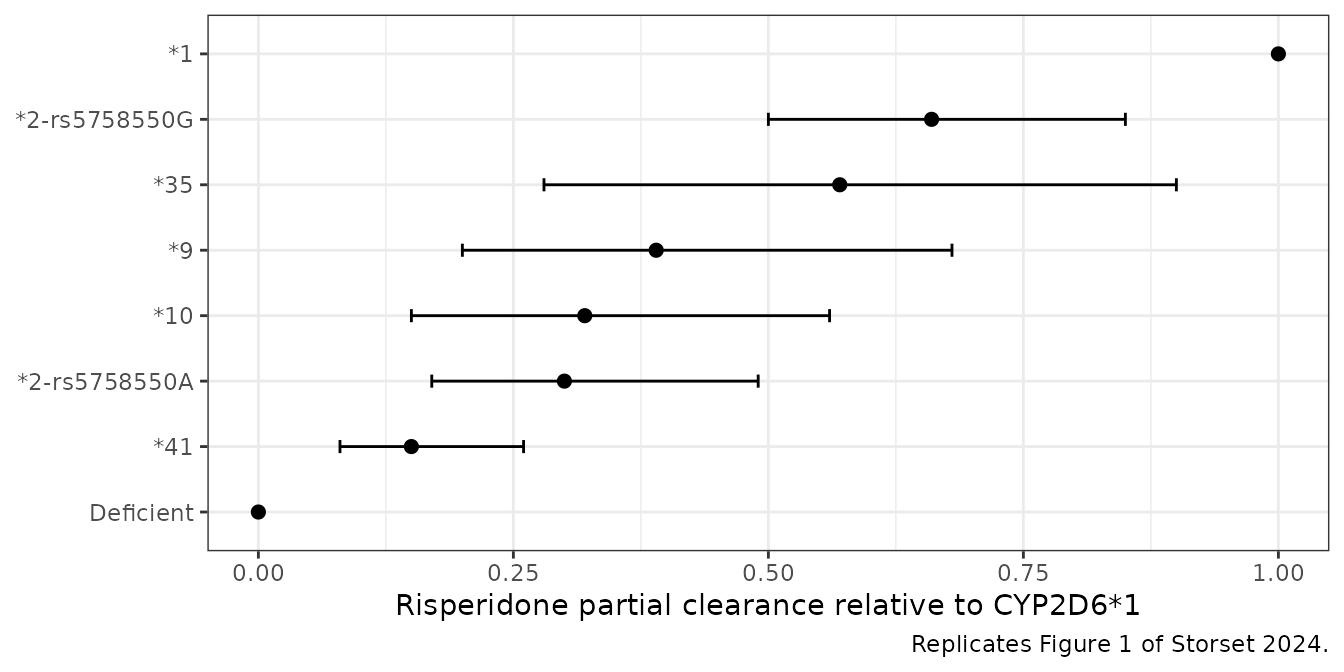
Typical metabolic ratio by diplotype (Figure 2)
Figure 2 overlays a horizontal line per diplotype: the model-predicted 9-hydroxyrisperidone / risperidone metabolic ratio for a typical subject aged 37 years, NFIB TT, sampled 13 h after the last dose. The line heights were digitised by the maintainers from the published figure (one pixel is 0.3 ratio units). The figure does not state the dosing frequency or dose; the ratio does not depend on dose because the model is linear, and the digitised values are reproduced with twice-daily dosing (last dose 13 h before the sample, the next dose not yet taken), so that regimen is used here. Once-daily dosing gives ratios about 20 % lower.
fig2 <- data.frame(
  diplotype = c("*1/*1", "*1/*2-G", "*1/*35", "*1/*9", "*1/*10", "*1/*2-A",
                "*1/*41", "*2-G/*2-G", "*2-G/*35", "*2-G/*10", "*2-A/*2-G",
                "*2-G/*41", "*35/*35", "*35/*41", "*2-A/*2-A", "*2-A/*41",
                "*41/*41", "*1/def", "*2-G/def", "*35/def", "*9/def",
                "*10/def", "*2-A/def", "*41/def", "def/def"),
  published = c(16.16, 11.56, 10.48, 8.70, 8.13, 7.77, 6.59, 8.13, 7.20,
                5.41, 5.11, 4.20, 6.45, 3.57, 3.00, 2.44, 1.54, 5.40, 3.30,
                2.75, 1.95, 1.80, 1.58, 1.06, 0.60)
)

ii <- 12
n_dose <- 70
t_obs <- (n_dose - 1) * ii + 13
ev_fig2 <- lapply(seq_len(nrow(fig2)), function(i) {
  data.frame(
    id = i,
    time = c((seq_len(n_dose) - 1) * ii, t_obs),
    amt = c(rep(1.5, n_dose), 0),
    evid = c(rep(1L, n_dose), 0L),
    cmt = c(rep("depot", n_dose), "central"),
    dvid = c(rep(NA_integer_, n_dose), 1L)
  )
}) |>
  dplyr::bind_rows()
cov_fig2 <- cbind(
  data.frame(id = seq_len(nrow(fig2)), AGE = 37, SNP_NFIB_RS28379954 = 0),
  diplotype_covariates(fig2$diplotype)
)
ev_fig2 <- dplyr::left_join(ev_fig2, cov_fig2, by = "id")
sim_fig2 <- solve_typ(ev_fig2)
#> ℹ omega/sigma items treated as zero: 'etalcl', 'etalcl_9oh'
fig2$simulated <- sim_fig2 |>
  dplyr::filter(time == t_obs) |>
  dplyr::arrange(id) |>
  dplyr::mutate(mr = Cc_9oh / Cc) |>
  dplyr::pull(mr)
fig2$pct_diff <- 100 * (fig2$simulated - fig2$published) / fig2$published

knitr::kable(
  fig2 |>
    md_escape() |>
    dplyr::rename(
      "Diplotype" = diplotype,
      "Figure 2 (digitised)" = published,
      "Model" = simulated,
      "Difference (%)" = pct_diff
    ),
  digits = 2
)| Diplotype | Figure 2 (digitised) | Model | Difference (%) |
|---|---|---|---|
| *1/*1 | 16.16 | 15.40 | -4.71 |
| *1/*2-G | 11.56 | 11.07 | -4.25 |
| *1/*35 | 10.48 | 10.10 | -3.63 |
| *1/*9 | 8.70 | 8.35 | -4.00 |
| *1/*10 | 8.13 | 7.73 | -4.86 |
| *1/*2-A | 7.77 | 7.56 | -2.65 |
| *1/*41 | 6.59 | 6.37 | -3.41 |
| *2-G/*2-G | 8.13 | 7.73 | -4.86 |
| *2-G/*35 | 7.20 | 6.99 | -2.95 |
| *2-G/*10 | 5.41 | 5.16 | -4.59 |
| *2-A/*2-G | 5.11 | 5.03 | -1.57 |
| *2-G/*41 | 4.20 | 4.10 | -2.32 |
| *35/*35 | 6.45 | 6.29 | -2.48 |
| *35/*41 | 3.57 | 3.59 | 0.67 |
| *2-A/*2-A | 3.00 | 2.97 | -1.10 |
| *2-A/*41 | 2.44 | 2.26 | -7.45 |
| *41/*41 | 1.54 | 1.62 | 5.43 |
| *1/def | 5.40 | 5.30 | -1.94 |
| *2-G/def | 3.30 | 3.27 | -0.80 |
| *35/def | 2.75 | 2.82 | 2.51 |
| *9/def | 1.95 | 2.00 | 2.35 |
| *10/def | 1.80 | 1.70 | -5.32 |
| *2-A/def | 1.58 | 1.62 | 2.76 |
| *41/def | 1.06 | 1.06 | -0.46 |
| def/def | 0.60 | 0.55 | -9.06 |
fig2$diplotype <- factor(fig2$diplotype, levels = fig2$diplotype)
ggplot(fig2, aes(diplotype)) +
  geom_point(aes(y = published, shape = "Figure 2 (digitised)"), size = 2.5) +
  geom_point(aes(y = simulated, shape = "Model"), size = 2, colour = "steelblue") +
  scale_shape_manual(values = c(4, 16), name = NULL) +
  labs(x = "CYP2D6 diplotype", y = "9-hydroxyrisperidone / risperidone ratio",
       caption = "Replicates the model-predicted lines of Figure 2 of Storset 2024.") +
  theme_bw() +
  theme(axis.text.x = element_text(angle = 60, hjust = 1))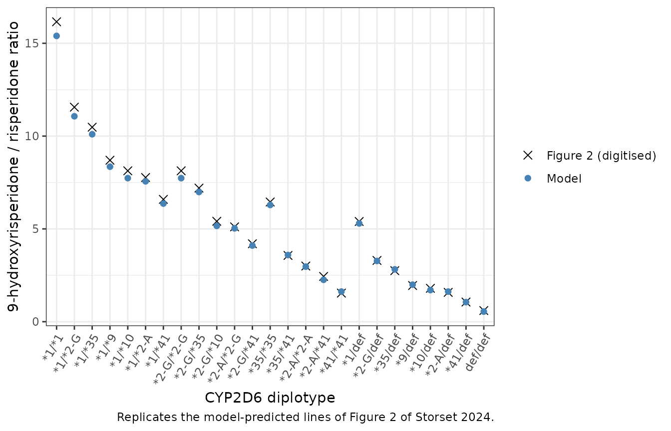
Both sides are deterministic typical values, so the remaining difference is digitisation error (one pixel is 5 % of the largest ratio and 50 % of the smallest) plus any difference in the dosing regimen the authors used.
Stochastic metabolic ratio by diplotype
A cohort of 100 subjects per diplotype for six common diplotypes (Supplementary Table S1) was simulated with between-subject variability, 1.5 mg twice daily, and a sample 13 h after the last dose. Ages were drawn from a log-normal distribution matching the cohort median of 37 years and truncated to the observed 18-89 range; NFIB C carriage was drawn at the cohort carrier frequency (53 C alleles of 1018 genotyped, about 10 % carriers under Hardy-Weinberg). The raw observed median metabolic ratios from Supplementary Table S1 are shown for orientation. They are medians of the per-subject median observed ratio over mixed dosing regimens and sampling times, so they are not expected to coincide with the simulated medians.
set.seed(20241)
rxode2::rxSetSeed(20241)
dips <- c("*1/*1", "*1/*2-G", "*1/*41", "*1/def", "*2-G/def", "def/def")
obs_s1 <- data.frame(
  diplotype = dips,
  n_subjects = c(82, 62, 26, 88, 37, 51),
  observed_median = c(25.5, 18.7, 8.0, 7.0, 3.8, 0.3)
)
n_per <- 100
cohort <- data.frame(
  id = seq_len(n_per * length(dips)),
  diplotype = rep(dips, each = n_per)
)
age <- exp(rnorm(nrow(cohort), log(37), 0.35))
cohort$AGE <- pmin(pmax(age, 18), 89)
cohort$SNP_NFIB_RS28379954 <- rbinom(nrow(cohort), 1, 0.10)
cohort <- cbind(cohort, diplotype_covariates(cohort$diplotype))

ev_mr <- lapply(cohort$id, function(i) {
  data.frame(
    id = i,
    time = c((seq_len(n_dose) - 1) * ii, t_obs),
    amt = c(rep(1.5, n_dose), 0),
    evid = c(rep(1L, n_dose), 0L),
    cmt = c(rep("depot", n_dose), "central"),
    dvid = c(rep(NA_integer_, n_dose), 1L)
  )
}) |>
  dplyr::bind_rows() |>
  dplyr::left_join(cohort, by = "id")

sim_mr <- rxode2::rxSolve(mod, ev_mr, returnType = "data.frame",
                          useLinCmt = FALSE, keep = "diplotype") |>
  dplyr::filter(time == t_obs) |>
  dplyr::mutate(mr = Cc_9oh / Cc)

mr_sum <- sim_mr |>
  dplyr::group_by(diplotype) |>
  dplyr::summarise(
    sim_median = median(mr),
    sim_p05 = quantile(mr, 0.05),
    sim_p95 = quantile(mr, 0.95),
    .groups = "drop"
  ) |>
  dplyr::left_join(obs_s1, by = "diplotype") |>
  dplyr::mutate(diplotype = factor(diplotype, levels = dips)) |>
  dplyr::arrange(diplotype)

knitr::kable(
  mr_sum |>
    md_escape() |>
    dplyr::rename(
      "Diplotype" = diplotype,
      "Simulated median" = sim_median,
      "Simulated 5th pct" = sim_p05,
      "Simulated 95th pct" = sim_p95,
      "Table S1 subjects" = n_subjects,
      "Table S1 observed median" = observed_median
    ),
  digits = 2
)| Diplotype | Simulated median | Simulated 5th pct | Simulated 95th pct | Table S1 subjects | Table S1 observed median |
|---|---|---|---|---|---|
| *1/*1 | 24.62 | 2.57 | 794.55 | 82 | 25.5 |
| *1/*2-G | 13.37 | 2.51 | 192.47 | 62 | 18.7 |
| *1/*41 | 8.42 | 1.61 | 118.61 | 26 | 8.0 |
| *1/def | 5.24 | 1.18 | 55.66 | 88 | 7.0 |
| *2-G/def | 3.44 | 0.87 | 28.01 | 37 | 3.8 |
| def/def | 0.55 | 0.19 | 1.90 | 51 | 0.3 |
ggplot(sim_mr, aes(factor(diplotype, levels = dips), mr)) +
  geom_boxplot(outlier.size = 0.6) +
  geom_point(data = mr_sum, aes(diplotype, observed_median),
             colour = "firebrick", shape = 18, size = 3) +
  scale_y_log10() +
  labs(x = "CYP2D6 diplotype", y = "9-hydroxyrisperidone / risperidone ratio",
       caption = "Boxes: simulated. Red diamonds: observed medians, Supplementary Table S1.") +
  theme_bw()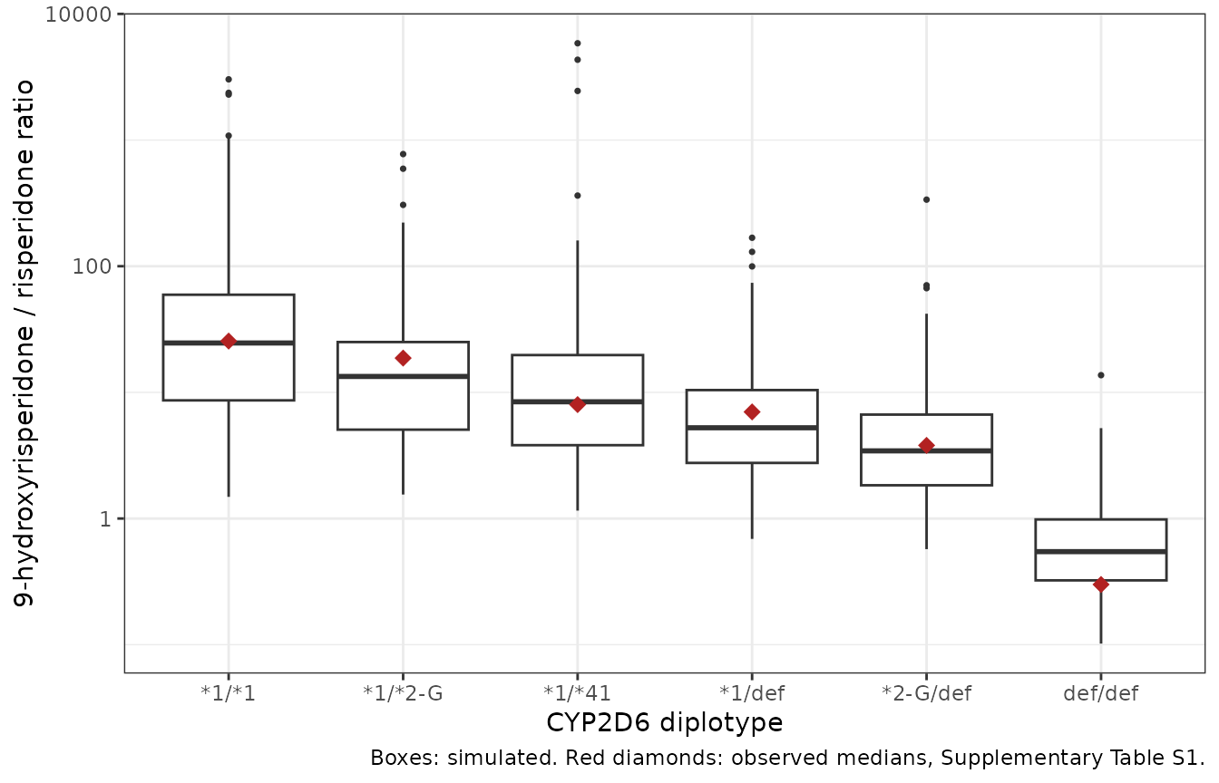
The simulated medians follow the CYP2D6 activity sum. The check below uses only the three diplotypes whose activities are far apart (2, 1 and 0 units of *1); adjacent diplotypes such as *1/*41 (1.15 units) and *1/def (1 unit) are closer than the Monte Carlo error of a 100-subject median under 86 % CV clearance variability, so their order is not asserted.
med <- setNames(mr_sum$sim_median, as.character(mr_sum$diplotype))
stopifnot(med[["*1/*1"]] > med[["*1/def"]], med[["*1/def"]] > med[["def/def"]])
Age effect on the active moiety
The Discussion states that the total active moiety (risperidone +
9-hydroxyrisperidone) is predicted to be more than doubled at 75 years
and older compared with a 30-year-old. The typical-value steady-state
average concentrations below (*1/*1, NFIB TT) use
Css,avg = dose rate / CL for each analyte; the metabolite
term is exact because all parent clearance forms metabolite in the
apparent parameterisation.
ages <- c(30, 75, 80, 85)
cl_age <- data.frame(id = seq_along(ages), time = 0, amt = 0, evid = 0L,
                     cmt = "central", dvid = 1L, AGE = ages,
                     SNP_NFIB_RS28379954 = 0)
cl_age <- cbind(cl_age, diplotype_covariates(rep("*1/*1", length(ages))))
s_age <- solve_typ(cl_age)
#> ℹ omega/sigma items treated as zero: 'etalcl', 'etalcl_9oh'
dose_rate <- 3 / 24
moiety <- data.frame(
  age = ages,
  cl = s_age$cl,
  cl_9oh = s_age$cl_9oh,
  css_moiety = 1000 * (dose_rate / s_age$cl + dose_rate / s_age$cl_9oh)
)
moiety$ratio_vs_30 <- moiety$css_moiety / moiety$css_moiety[1]
knitr::kable(
  moiety |>
    dplyr::rename(
      "Age (years)" = age,
      "Risperidone CL/F (L/h)" = cl,
      "9-OH CL (L/h)" = cl_9oh,
      "Active moiety Css,avg at 3 mg/day (ng/mL)" = css_moiety,
      "Ratio to age 30" = ratio_vs_30
    ),
  digits = 2
)| Age (years) | Risperidone CL/F (L/h) | 9-OH CL (L/h) | Active moiety Css,avg at 3 mg/day (ng/mL) | Ratio to age 30 |
|---|---|---|---|---|
| 30 | 50.60 | 8.00 | 18.10 | 1.00 |
| 75 | 31.93 | 4.26 | 33.29 | 1.84 |
| 80 | 29.65 | 3.74 | 37.67 | 2.08 |
| 85 | 27.37 | 3.22 | 43.43 | 2.40 |
stopifnot(
  moiety$ratio_vs_30[moiety$age == 80] > 2,
  moiety$ratio_vs_30[moiety$age == 75] > 1.8
)
The ratio is 1.84 at exactly 75 years and 2.08 at 80 years, consistent with “more than doubled in subjects 75 years and older” as a statement about that age group rather than about age 75 itself.
Steady-state NCA by metabolizer group
A stochastic cohort of 100 subjects per group (normal *1/*1, intermediate *1/def, poor def/def) was dosed 1.5 mg twice daily to steady state and sampled densely over the last dosing interval. PKNCA computes the dosing-interval AUC for each analyte. Because the paper reports no NCA, the check is internal: at steady state AUCtau equals dose / CL for risperidone and dose / CLmet for 9-hydroxyrisperidone (all parent clearance forms metabolite), using each subject’s own simulated clearances.
rxode2::rxSetSeed(20242)
groups <- c("*1/*1" = "Normal (*1/*1)", "*1/def" = "Intermediate (*1/def)",
            "def/def" = "Poor (def/def)")
n_grp <- 100
nca_cohort <- data.frame(
  id = seq_len(n_grp * length(groups)),
  diplotype = rep(names(groups), each = n_grp)
)
nca_cohort$treatment <- unname(groups[nca_cohort$diplotype])
nca_cohort$AGE <- 30
nca_cohort$SNP_NFIB_RS28379954 <- 0
nca_cohort <- cbind(nca_cohort, diplotype_covariates(nca_cohort$diplotype))

n_ss <- 120
t_last <- (n_ss - 1) * ii
obs_t <- t_last + seq(0, ii, by = 0.25)
ev_nca <- lapply(nca_cohort$id, function(i) {
  data.frame(
    id = i,
    time = c((seq_len(n_ss) - 1) * ii, obs_t),
    amt = c(rep(1.5, n_ss), rep(0, length(obs_t))),
    evid = c(rep(1L, n_ss), rep(0L, length(obs_t))),
    cmt = c(rep("depot", n_ss), rep("central", length(obs_t))),
    dvid = c(rep(NA_integer_, n_ss), rep(1L, length(obs_t)))
  )
}) |>
  dplyr::bind_rows() |>
  dplyr::left_join(nca_cohort, by = "id") |>
  dplyr::arrange(id, time, -evid)

sim_nca <- rxode2::rxSolve(mod, ev_nca, returnType = "data.frame",
                           useLinCmt = FALSE, keep = "treatment") |>
  dplyr::filter(time >= t_last) |>
  dplyr::mutate(tad = time - t_last)
nca_long <- sim_nca |>
  dplyr::select(id, treatment, tad, Cc, Cc_9oh) |>
  tidyr::pivot_longer(c(Cc, Cc_9oh), names_to = "analyte", values_to = "conc") |>
  dplyr::filter(!is.na(conc))
dose_df <- nca_long |>
  dplyr::distinct(id, treatment, analyte) |>
  dplyr::mutate(tad = 0, dose = 1.5)

conc_obj <- PKNCA::PKNCAconc(nca_long, conc ~ tad | treatment + analyte + id)
dose_obj <- PKNCA::PKNCAdose(dose_df, dose ~ tad | treatment + analyte + id)
intervals <- data.frame(start = 0, end = ii, auclast = TRUE, cmax = TRUE,
                        tmax = TRUE, cmin = TRUE, cav = TRUE)
nca_res <- PKNCA::pk.nca(PKNCA::PKNCAdata(conc_obj, dose_obj, intervals = intervals))
nca_tab <- as.data.frame(nca_res)

summary(nca_res)
#>  start end             treatment analyte   N     auclast        cmax
#>      0  12 Intermediate (*1/def)      Cc 100 58.4 [78.3] 7.08 [49.5]
#>      0  12 Intermediate (*1/def)  Cc_9oh 100  193 [43.1] 16.9 [40.0]
#>      0  12        Normal (*1/*1)      Cc 100 30.7 [97.9] 4.88 [49.6]
#>      0  12        Normal (*1/*1)  Cc_9oh 100  182 [53.1] 16.8 [44.9]
#>      0  12        Poor (def/def)      Cc 100  357 [84.4] 31.9 [76.7]
#>      0  12        Poor (def/def)  Cc_9oh 100  189 [42.6] 15.9 [42.1]
#>         cmin               tmax         cav
#>   2.62 [174]  1.50 [1.00, 1.50] 4.87 [78.3]
#>  14.6 [50.1]  5.50 [4.00, 6.00] 16.0 [43.1]
#>  0.620 [970] 1.25 [0.750, 1.50] 2.56 [97.9]
#>  12.4 [76.6]  5.25 [3.00, 6.25] 15.1 [53.1]
#>  27.1 [96.0]  1.50 [1.50, 1.75] 29.7 [84.4]
#>  15.5 [43.5]  6.00 [5.25, 9.50] 15.7 [42.6]
#>
#> Caption: auclast, cmax, cmin, cav: geometric mean and geometric coefficient of variation; tmax: median and range; N: number of subjects
cl_sub <- sim_nca |>
  dplyr::distinct(id, cl, cl_9oh)
auc_chk <- nca_tab |>
  dplyr::filter(PPTESTCD == "auclast") |>
  dplyr::left_join(cl_sub, by = "id") |>
  dplyr::mutate(
    expected = 1000 * 1.5 / ifelse(analyte == "Cc", cl, cl_9oh),
    pct_diff = 100 * (PPORRES - expected) / expected
  )
auc_sum <- auc_chk |>
  dplyr::group_by(treatment, analyte) |>
  dplyr::summarise(
    median_auc = median(PPORRES),
    median_pct_diff = median(pct_diff),
    p90_abs_pct_diff = quantile(abs(pct_diff), 0.9),
    .groups = "drop"
  )
knitr::kable(
  auc_sum |>
    md_escape() |>
    dplyr::rename(
      "Group" = treatment,
      "Analyte" = analyte,
      "Median AUCtau (ng*h/mL)" = median_auc,
      "Median % diff vs dose/CL" = median_pct_diff,
      "90th pct |% diff|" = p90_abs_pct_diff
    ),
  digits = 2
)| Group | Analyte | Median AUCtau (ng*h/mL) | Median % diff vs dose/CL | 90th pct |% diff| |
|---|---|---|---|---|
| Intermediate (*1/def) | Cc | 65.67 | -0.07 | 0.21 |
| Intermediate (*1/def) | Cc_9oh | 202.44 | 0.00 | 0.00 |
| Normal (*1/*1) | Cc | 30.85 | -0.16 | 0.47 |
| Normal (*1/*1) | Cc_9oh | 175.15 | 0.00 | 0.00 |
| Poor (def/def) | Cc | 374.77 | -0.02 | 0.11 |
| Poor (def/def) | Cc_9oh | 194.76 | 0.00 | 0.11 |
The dosing-interval AUC matches dose / CL to within the trapezoid error for both analytes in every group, confirming the parent-to-metabolite routing and the steady-state behaviour of the additive clearance.
Assumptions and deviations
-
CYP2D6 encoding. The paper assigns each subject a
diplotype and sums the per-allele partial clearances. The model receives
the diplotype as heterozygote / homozygote indicator pairs per allele
category and counts copies as
HET + 2 * HOM. Deficient alleles (*3-*6, fixed at zero clearance in the paper) need no column. Gene duplications cannot be expressed this way: the two subjects with three alleles (*1/*1xN and *2-G/*2-G xN, Table 1 footnote) would be encoded as their two-copy diplotype. -
CYP2D6*10. In this cohort *10 is a star-allele call
from the routine panel in which *4 (which also carries the rs1065852
variant) is called separately as deficient;
CYP2D6_STAR10_HET/_HOMtherefore mean *10 copies, not raw rs1065852 genotype. - CYP2D6*1 includes three *1-rs5758550G alleles that the paper merged with *1-rs5758550A. Heterozygous *1/*2 with rs5758550 A/G were assumed by the authors to be *1-rs5758550A/*2-rs5758550G (Discussion).
-
NFIB unknown genotype. Six of 1024 NFIB alleles
were undetermined. The final model has no separate unknown category, so
undetermined genotype is coded as NFIB-T
(
SNP_NFIB_RS28379954 = 0). -
Age function. The Table 2 footnote form
1 - CLage x (Age - AgeBP)forAge >= AgeBPis written as1 + e_age_cl * max(AGE - age_hinge, 0)with the signed Table 2 reduction per year (-0.9 % and -1.3 %). -
Between-subject variability. Table 2 reports 86 %
and 49 % CV; these were converted with
omega^2 = log(1 + CV^2)(the Methods define CV assqrt(exp(omega^2) - 1)). The covariance uses the reported correlation of 0.43. -
Residual error. Table 2 reports the proportional
errors as percentages (58 % and 38 %) and the additive error as 0.06
ng/mL; these are taken as standard deviations. The combined error
follows the Methods equation
Obs = Pred (1 + eps1) + eps2, which is nlmixr2’s default combined form. -
Concentration units. The assay reports nmol/L but
Table 2 gives the additive error in ng/mL, so the model works in mg
doses and ng/mL. The metabolite parameters are apparent
(
/(F x fmet)); the unidentified fraction metabolised, and the 4 % molecular-weight difference between risperidone and 9-hydroxyrisperidone, are absorbed into them, so the 9-hydroxyrisperidone output is on the scale the authors fitted. - Figure 2 regimen. The figure states age 37, NFIB TT and 13 h after dose but not the dosing frequency; twice-daily dosing reproduces the digitised lines and was used.
-
Not retained. Sex (p >= 0.23) and CYP3A4*22 (p =
0.31) were tested but not retained and are documented under
covariatesDataExcluded. - Lower limit of detection. Concentrations below the detection limit were imputed at half the limit during fitting (Methods); this affects the fit, not the model structure.