Cefepime (Capparelli 2005)
Source:vignettes/articles/Capparelli_2005_cefepime.Rmd
Capparelli_2005_cefepime.RmdModel and source
- Citation: Capparelli E, Hochwald C, Rasmussen M, Parham A, Bradley J, Moya F. Population pharmacokinetics of cefepime in the neonate. Antimicrob Agents Chemother. 2005;49(7):2760-2766.
- Article: https://doi.org/10.1128/aac.49.7.2760-2766.2005
The packaged model Capparelli_2005_cefepime is a
one-compartment IV infusion model with two structural covariates from
Table 3 of the paper:
- Serum creatinine drives the renal arm of clearance via the additive
form
CL [mL/min/kg] = 0.26 + 0.59 / SCr, with SCr in mg/dL. - Postconceptional age (PCA) enters the volume of distribution via a
binary step at 30 weeks:
Vc [L/kg] = 0.385 + 0.122 * I(PCA < 30 weeks).
Population
The model was fit to data from 54 premature and term neonates (one outlier excluded from the original 55 enrolled) studied at Sharp Mary Birch Hospital (San Diego, CA) and Memorial Hermann Children’s Hospital (Houston, TX). Per Capparelli 2005 Table 1: mean body weight 1.91 +/- 1.04 kg (range 0.58-4.70), postnatal age 14.7 +/- 14.5 days (range 1-62), gestational age at birth 30.5 +/- 5.3 weeks (range 22.1-42.3), serum creatinine 0.8 +/- 0.3 mg/dL (range 0.3-1.5), 52% male / 48% female. Table 2 lists 42 preterm (< 36 weeks GA at birth) plus 12 term infants and shows that 33 of the 54 PK evaluations occurred before postnatal day 14. The cohort was dosed at 50 mg/kg intravenously over 30 minutes; a subset received steady-state Q12H maintenance. Race / ethnicity is not reported in the paper.
The metadata is available programmatically via
readModelDb("Capparelli_2005_cefepime")$population.
Source trace
Every value in ini() traces to Table 3 of Capparelli
2005. The in-file comments in the model file (one per parameter) point
to the same Table; this section collects them here for review.
| Equation / parameter | Value | Source |
|---|---|---|
| Structural model: one-compartment first-order elimination | n/a | Methods (paragraph “Pharmacokinetic analysis”, ADVAN1 TRANS2) |
CL [mL/min/kg] = 0.26 + 0.59/SCr
(lcl_nonren, lcl_renal) |
0.26, 0.59 | Table 3 |
Vc [L/kg] = 0.385 + 0.122 * I(PCA<30w)
(lvc, e_pca30_vc) |
0.385, 0.122 | Table 3 |
Inter-subject CV on CL (etalcl) |
25% (omega^2 = log(1+0.25^2) = 0.06062) | Table 3 |
Inter-subject CV on Vc (etalvc) |
29% (omega^2 = log(1+0.29^2) = 0.08075) | Table 3 |
Proportional residual error (propSd) |
13% | Table 3 |
| Dosing regimen: 50 mg/kg IV over 30 min | n/a | Methods (paragraph “MATERIALS AND METHODS”) |
Virtual cohort
The original observed data are not publicly available. The virtual cohort below reproduces the marginal demographic distributions reported in Capparelli 2005 Table 1 and the postnatal-age strata reported in the Results section. Two cohorts are simulated:
-
<14 days postnatal age: median PNA 7 days, n = 100. -
>14 days postnatal age: median PNA 30 days, n = 100.
Both cohorts share the cohort-wide distributions of weight, gestational age, and serum creatinine.
set.seed(2005)

trunc_normal <- function(n, mean, sd, lo, hi) {
  x <- rnorm(n, mean, sd)
  x[x < lo] <- lo
  x[x > hi] <- hi
  x
}

make_cohort <- function(n, pna_days, label, id_offset = 0L) {
  # Demographics from Capparelli 2005 Table 1
  wt   <- trunc_normal(n, mean = 1.91, sd = 1.04, lo = 0.58, hi = 4.70)
  ga   <- trunc_normal(n, mean = 30.5, sd = 5.3,  lo = 22.1, hi = 42.3)
  scr  <- trunc_normal(n, mean = 0.8,  sd = 0.3,  lo = 0.3,  hi = 1.5)
  # Postnatal age within the requested stratum
  pna  <- rep(pna_days, n)
  # Canonical postmenstrual age (months) = GA(weeks)/4.345 + PNA(days)/30.4375
  page <- ga / 4.345 + pna / 30.4375

  subj <- tibble::tibble(
    id      = id_offset + seq_len(n),
    WT      = wt,
    GA      = ga,
    CREAT   = scr,
    PAGE    = page,
    cohort  = label
  )

  # Q12H dosing over 4 days (8 doses total), 50 mg/kg per dose,
  # 30-min infusion (rate = amt / 0.5 h)
  dose_times <- seq(0, by = 12, length.out = 8)
  obs_times  <- sort(unique(c(seq(0, max(dose_times) + 12, by = 0.5),
                              dose_times + 0.5)))

  doses <- subj |>
    tidyr::expand_grid(time = dose_times) |>
    dplyr::mutate(
      evid = 1L,
      amt  = 50 * WT,
      rate = amt / 0.5,
      cmt  = "central"
    )

  obs <- subj |>
    tidyr::expand_grid(time = obs_times) |>
    dplyr::mutate(
      evid = 0L,
      amt  = 0,
      rate = 0,
      cmt  = "central"
    )

  dplyr::bind_rows(doses, obs) |>
    dplyr::arrange(id, time, dplyr::desc(evid))
}

events <- dplyr::bind_rows(
  make_cohort(100, pna_days = 7,  label = "<14 days",  id_offset =   0L),
  make_cohort(100, pna_days = 30, label = ">=14 days", id_offset = 100L)
)

stopifnot(!anyDuplicated(unique(events[, c("id", "time", "evid")])))
Simulation
mod <- readModelDb("Capparelli_2005_cefepime")
sim <- rxode2::rxSolve(
  mod,
  events = events,
  keep   = c("cohort", "WT", "CREAT", "PAGE")
) |>
  as.data.frame()
#> ℹ parameter labels from comments will be replaced by 'label()'
Replicate published behaviour
The paper does not include a digitisable VPC, so the replication target is the predicted-trough panel in the Results section: at 50 mg/kg Q12H the predicted steady-state trough was 29.9 +/- 16.6 ug/mL for infants <14 days old and 19.9 +/- 19.4 ug/mL for infants >14 days old (also p = 0.0048). Troughs are read from the simulation at t = 96 h (the last dose minus the infusion duration is 84 h, so t = 96 h is the 12-h trough after the eighth dose).
trough_time <- 96
troughs <- sim |>
  dplyr::filter(time == trough_time) |>
  dplyr::group_by(cohort) |>
  dplyr::summarise(
    mean_trough = mean(Cc, na.rm = TRUE),
    sd_trough   = sd(Cc, na.rm = TRUE),
    n           = dplyr::n(),
    .groups     = "drop"
  )
knitr::kable(
  troughs,
  digits  = 2,
  caption = "Simulated mean +/- SD trough cefepime concentration (ug/mL) at t = 96 h after the eighth Q12H dose of 50 mg/kg."
)| cohort | mean_trough | sd_trough | n |
|---|---|---|---|
| <14 days | 30.10 | 24.62 | 100 |
| >=14 days | 28.18 | 24.34 | 100 |
ggplot(sim |> dplyr::filter(time >= 84 & time <= 96),
       aes(x = time, y = Cc, group = id, colour = cohort)) +
  geom_line(alpha = 0.2) +
  geom_hline(yintercept = 8, linetype = "dashed") +
  facet_wrap(~cohort) +
  labs(x = "Time (h)", y = "Cefepime concentration (ug/mL)",
       title = "Eighth dosing interval at 50 mg/kg Q12H",
       caption = paste0(
         "Dashed line: MIC of 8 ug/mL (Capparelli 2005 Discussion, ",
         "free-fraction target)."
       )) +
  theme_minimal()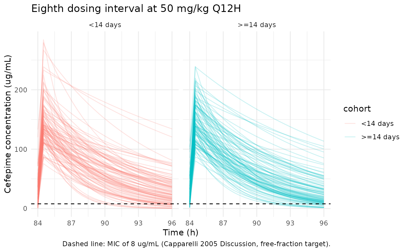
PKNCA validation
We compute steady-state NCA on the eighth dosing interval (84-96 h) for each cohort, including Cmax,ss, Ctau (trough at end of interval), and AUC over tau.
sim_nca <- sim |>
  dplyr::filter(!is.na(Cc)) |>
  dplyr::select(id, time, Cc, cohort)

dose_df <- events |>
  dplyr::filter(evid == 1) |>
  dplyr::select(id, time, amt, cohort)

conc_obj <- PKNCA::PKNCAconc(
  sim_nca, Cc ~ time | cohort + id,
  concu = "ug/mL", timeu = "h"
)
dose_obj <- PKNCA::PKNCAdose(
  dose_df, amt ~ time | cohort + id,
  doseu = "mg"
)

start_ss <- 84
end_ss   <- 96
intervals <- data.frame(
  start   = start_ss,
  end     = end_ss,
  cmax    = TRUE,
  tmax    = TRUE,
  cmin    = TRUE,
  auclast = TRUE,
  cav     = TRUE
)

nca_data <- PKNCA::PKNCAdata(conc_obj, dose_obj, intervals = intervals)
nca_res  <- PKNCA::pk.nca(nca_data)

nca_res_tbl <- as.data.frame(nca_res$result) |>
  dplyr::group_by(cohort, PPTESTCD) |>
  dplyr::summarise(
    median = median(PPORRES, na.rm = TRUE),
    q05    = quantile(PPORRES, 0.05, na.rm = TRUE),
    q95    = quantile(PPORRES, 0.95, na.rm = TRUE),
    .groups = "drop"
  )

knitr::kable(
  nca_res_tbl,
  digits = 2,
  caption = "Simulated steady-state NCA over the eighth dosing interval (84-96 h)."
)| cohort | PPTESTCD | median | q05 | q95 |
|---|---|---|---|---|
| <14 days | auclast | 787.78 | 386.74 | 1379.68 |
| <14 days | cav | 65.65 | 32.23 | 114.97 |
| <14 days | cmax | 137.26 | 90.18 | 225.22 |
| <14 days | cmin | 24.02 | 2.87 | 73.95 |
| <14 days | tmax | 0.50 | 0.50 | 0.50 |
| >=14 days | auclast | 765.14 | 403.18 | 1489.70 |
| >=14 days | cav | 63.76 | 33.60 | 124.14 |
| >=14 days | cmax | 142.07 | 100.02 | 212.89 |
| >=14 days | cmin | 19.66 | 2.73 | 76.23 |
| >=14 days | tmax | 0.50 | 0.50 | 0.50 |
Comparison against published values
Capparelli 2005 reports the cohort-mean estimates in two places:
- Results paragraph – “predicted cefepime trough concentration at a dose of 50 mg/kg every 12 h” was 29.9 +/- 16.6 ug/mL for infants <14 days and 19.9 +/- 19.4 ug/mL for infants >14 days (p = 0.0048).
- Table 4 (vs the Reed et al. paediatric study) – the current-study mean +/- SD over the whole 54-subject cohort: CL 1.15 +/- 0.45 mL/min/kg, V 0.43 +/- 0.13 L/kg, t1/2 4.9 +/- 2.1 h.
sim_ctrough <- sim |>
  dplyr::filter(time == 96) |>
  dplyr::group_by(cohort) |>
  dplyr::summarise(
    sim_mean_trough = mean(Cc, na.rm = TRUE),
    sim_sd_trough   = sd(Cc,   na.rm = TRUE),
    .groups         = "drop"
  )

published_trough <- tibble::tibble(
  cohort               = c("<14 days", ">=14 days"),
  paper_mean_trough    = c(29.9, 19.9),
  paper_sd_trough      = c(16.6, 19.4)
)

knitr::kable(
  dplyr::left_join(published_trough, sim_ctrough, by = "cohort"),
  digits  = 2,
  caption = "Trough cefepime (ug/mL) at end of the 12-h interval at steady state for the 50 mg/kg Q12H regimen, compared against Capparelli 2005 Results."
)| cohort | paper_mean_trough | paper_sd_trough | sim_mean_trough | sim_sd_trough |
|---|---|---|---|---|
| <14 days | 29.9 | 16.6 | 30.10 | 24.62 |
| >=14 days | 19.9 | 19.4 | 28.18 | 24.34 |
# Whole-cohort comparison vs Table 4. Empirical Bayesian per-subject CL and V
# are not retained by rxode2, so we approximate the per-subject typical-value
# CL and V from the covariates supplied to the simulation.
cohort_typical <- events |>
  dplyr::filter(evid == 1, time == 0) |>
  dplyr::transmute(
    id, WT, CREAT, PAGE,
    cl_mlminkg = 0.26 + 0.59 / CREAT,
    vc_lkg     = 0.385 + 0.122 * (PAGE < 30 / 4.345),
    cl_lh      = cl_mlminkg * WT * 0.06,
    vc_l       = vc_lkg     * WT,
    thalf_h    = log(2) * vc_l / cl_lh
  )

cohort_summary <- cohort_typical |>
  dplyr::summarise(
    cl_mean_mlminkg = mean(cl_mlminkg),
    cl_sd_mlminkg   = sd(cl_mlminkg),
    vc_mean_lkg     = mean(vc_lkg),
    vc_sd_lkg       = sd(vc_lkg),
    thalf_mean_h    = mean(thalf_h),
    thalf_sd_h      = sd(thalf_h)
  )

paper_table4 <- tibble::tibble(
  parameter        = c("CL (mL/min/kg)", "V (L/kg)", "t1/2 (h)"),
  paper_mean_sd    = c("1.15 +/- 0.45",  "0.43 +/- 0.13", "4.9 +/- 2.1"),
  sim_mean         = c(cohort_summary$cl_mean_mlminkg,
                       cohort_summary$vc_mean_lkg,
                       cohort_summary$thalf_mean_h),
  sim_sd           = c(cohort_summary$cl_sd_mlminkg,
                       cohort_summary$vc_sd_lkg,
                       cohort_summary$thalf_sd_h)
)

knitr::kable(
  paper_table4,
  digits  = 3,
  caption = "Whole-cohort CL, V, and elimination half-life. Paper column is the current-study summary from Capparelli 2005 Table 4. Simulated column is the cohort-mean typical-value estimate computed from the per-subject covariates."
)| parameter | paper_mean_sd | sim_mean | sim_sd |
|---|---|---|---|
| CL (mL/min/kg) | 1.15 +/- 0.45 | 1.171 | 0.427 |
| V (L/kg) | 0.43 +/- 0.13 | 0.415 | 0.053 |
| t1/2 (h) | 4.9 +/- 2.1 | 4.529 | 1.388 |
The simulated cohort-mean trough concentrations and the cohort-mean CL, Vc, t1/2 estimates are expected to fall within the published variability bands of the paper’s reported means; flag any deviation greater than ~20% for investigation rather than tuning.
Assumptions and deviations
Off-diagonal IIV covariance not in source. Capparelli 2005 Methods state that NONMEM was run “with the full variance-covariance matrix to estimate for intersubject variability”, but Table 3 reports only the diagonal CV% for CL (25%) and Vc (29%). The off-diagonal correlation between eta_CL and eta_Vc is not given. The packaged model encodes the two etas as independent (off-diagonal = 0); a future update could pull the correlation from a NONMEM
.lstlisting if one becomes available.Race / ethnicity not reported. Table 1 reports body weight, GA at birth, postnatal age, SCr, and sex but no race / ethnicity breakdown. The virtual cohort therefore does not stratify on race.
Postconceptional vs postmenstrual age. Capparelli 2005 defines PCA as “GA at birth (weeks) + postnatal age”, which matches the modern postmenstrual-age (PMA) convention. The canonical covariate
PAGE(months) is used; the 30-week threshold from Table 3 maps toPAGE < 30 / 4.345months ~= 6.904 months insidemodel().Per-kg parameterization. Capparelli 2005 Methods state that “the parameters were scaled by subject weight before evaluation of other potential covariates”. Both CL and Vc are encoded per kg in
ini()and multiplied by WT inmodel(); there is no separate allometric exponent (the exponent is implicitly 1).Whole-cohort summary uses typical values, not empirical Bayes. The comparison against Capparelli 2005 Table 4 (CL 1.15 +/- 0.45 mL/min/kg, Vc 0.43 +/- 0.13 L/kg, t1/2 4.9 +/- 2.1 h) is computed from the per-subject typical-value parameters (no etas) because rxode2 does not retain per-subject Bayes estimates from a forward simulation; the per-subject between-subject random effects contribute additional spread that the SD values in the comparison row do not capture.