Aguiar_2021_ustekinumab • nlmixr2lib

library(nlmixr2lib)
library(rxode2)
#> rxode2 5.0.2 using 2 threads (see ?getRxThreads)
#>   no cache: create with `rxCreateCache()`
library(dplyr)
#> 
#> Attaching package: 'dplyr'
#> The following objects are masked from 'package:stats':
#> 
#>     filter, lag
#> The following objects are masked from 'package:base':
#> 
#>     intersect, setdiff, setequal, union
library(tidyr)
library(ggplot2)
library(PKNCA)
#> 
#> Attaching package: 'PKNCA'
#> The following object is masked from 'package:stats':
#> 
#>     filter

Ustekinumab popPK-PD in Crohn’s disease (Aguiar 2021)

Replicate the population pharmacokinetic-pharmacodynamic model reported by Aguiar Zdovc et al. (2021) for ustekinumab in adults with Crohn’s disease. Ustekinumab is an IgG1k monoclonal antibody that binds the p40 subunit shared by interleukin-12 and interleukin-23. The structural model is a two-compartment quasi-equilibrium target-mediated drug disposition (QE-TMDD) model for the unbound drug and the unbound IL-12/IL-23 p40 target, both distributing in two-compartment systems and binding only in the central compartment, linked to fecal calprotectin via an indirect-response model in which the unbound target stimulates FC production.

Citation: Aguiar Zdovc J, Hanzel J, Kurent T, Sever N, Smrekar N, Kozelj M, Novak G, Stabuc B, Drobne D, Grabnar I. Ustekinumab Dosing Individualization in Crohn’s Disease Guided by a Population Pharmacokinetic-Pharmacodynamic Model. Pharmaceutics. 2021;13(10):1587. doi:10.3390/pharmaceutics13101587
Article: https://doi.org/10.3390/pharmaceutics13101587

Population

The Aguiar 2021 cohort comprised 57 adults with active Crohn’s disease starting ustekinumab at a single Slovenian tertiary referral center, followed for 32 weeks. Baseline demographics (Aguiar 2021 Table 1): 56% female; median age 49 years (IQR 32-56); median weight 70 kg (IQR 59-84); median fat-free mass 45 kg (IQR 39-62) derived per subject via the Janmahasatian 2005 model; median disease duration 14 years (IQR 7-22); 66.7% had been exposed to a prior biologic (38/57 prior anti-TNF; 10/57 prior vedolizumab); 77.2% had endoscopically active luminal disease at baseline; median serum CRP 3 mg/L (IQR 3-11), albumin 43 g/L (IQR 41-44), fecal calprotectin 134 mg/kg (IQR 53-213). FCGR3A rs396991 genotype distribution: V/V 8.8% (5/57), V/F 54.4% (31/57), F/F 36.8% (21/57).

Standard ustekinumab dosing (which the simulations below use) is weight-tiered IV induction (260 mg if WT $\le$ 55 kg, 390 mg if 55 < WT $\le$ 85 kg, 520 mg if WT > 85 kg) at week 0, followed by 90 mg subcutaneous maintenance every 8 weeks.

The same demographics are available programmatically via the model’s metadata (readModelDb("Aguiar_2021_ustekinumab")$population).

Source trace

The per-parameter origin is recorded as an in-file comment next to each ini() entry in inst/modeldb/specificDrugs/Aguiar_2021_ustekinumab.R. The table below collects them in one place. Concentrations are in nmol/L; the source paper converted ustekinumab concentrations to nmol/L using a molecular weight of 149 kDa (Aguiar 2021 Methods section 2.3).

Parameter / equation	Value	Source
`ka`	0.381 /day	Table 2 final-model Ka
`CL` (typical, reference covariates)	0.277 L/day	Table 2 final-model CL
`Vc` (reference FFM = 45 kg)	3.57 L	Table 2 final-model Vc
`Vp` (reference FFM = 45 kg)	3.30 L	Table 2 final-model Vp
`Q`	1.89 L/day	Table 2 final-model Q
`F` (V/F or F/F)	0.710 (logit 0.8954)	Table 2 final-model F (V/F, F/F)
`F` (V/V)	0.888 (logit 2.0705)	Table 2 final-model F (V/V)
FFM effect on CL	power exponent 0.598, reference 45 kg	Table 2 footnote a
FFM effect on Vc, Vp	power exponents 0.590 (Vc), 0.586 (Vp), reference 45 kg	Table 2 footnotes b, c
ALB linear effect on CL	(1 - 0.0165 * (ALB - 43))	Table 2 footnote a
Bio-naive effect on CL	(1 - 0.227 * bio_naive); bio_naive = 1 - PRIOR_BIO	Table 2 footnote a
FCGR3A V/V effect on F	logit shift 1.1751	Table 2 final-model
`Ksyn` (typical, reference CRP)	9.86e-9 nmol/L/day	Table 2 final-model Ksyn
`Kdeg`	9.26e-10 /day	Table 2 final-model Kdeg
CRP linear effect on Ksyn	(1 + 0.0846 * (CRP - 3))	Table 2 footnote d
`Vc-target`	2.44 L	Table 2 final-model Vc-target
`Qtarget`	0.493 L/day	Table 2 final-model Qtarget
`Vp-target`	11.0 L	Table 2 final-model Vp-target
`Kint`	2.83e-6 /day	Table 2 final-model Kint
`Kd`	0.168 nmol/L	Table 2 final-model Kd
`Kout`	0.0581 /day	Table 3 final-model Kout
`FC0` (no ulcers)	102 mg/kg	Table 3 final-model FC0
`FC0` (ulcers)	213 mg/kg	Table 3 final-model FC0 with ulcers
`Emax` (FC stim)	2.19 (= 219%)	Table 3 final-model Emax
`C50` (FC stim)	2.46 nmol/L	Table 3 final-model C50
Drug ODEs	n/a, see model file	Figure 1 + Table 2 footnotes
Target ODEs	n/a, see model file	Figure 1
Indirect-response PD	dFC/dt = (FC0 * Kout / stim_baseline) * stim_fc - Kout * FC	Table 3 footnote a
IIV CL	omega^2 = log(0.18^2 + 1) = 0.03188	Table 2 (18.0% CV)
IIV Vc	omega^2 = log(0.0979^2 + 1) = 0.00954	Table 2 (9.79% CV)
IIV Vp	omega^2 = log(0.241^2 + 1) = 0.05645	Table 2 (24.1% CV)
IIV logit(F)	omega^2 = 0.173^2 = 0.02993	Table 2 (SD = 0.173 on logit scale)
IIV Ksyn	omega^2 = log(0.992^2 + 1) = 0.68522	Table 2 (99.2% CV)
IIV FC0	omega^2 = log(0.99^2 + 1) = 0.68309	Table 3 (99.0% CV)
Residual on Cc	additive 4.55 nmol/L + proportional 7.77%	Table 2
Residual on FC	proportional 57.3%	Table 3

Covariate column naming

Source column	Canonical column used here	Notes
FFM (kg)	`FFM`	Reference 45 kg (cohort median); derived per subject via Janmahasatian 2005.
Serum albumin	`ALB` (g/L)	Reference 43 g/L (cohort median).
C-reactive protein	`CRP` (mg/L)	Standard CRP assay; reference 3 mg/L (cohort median).
bio-naive (1 = no prior biologic)	`PRIOR_BIO` (1 = previously exposed)	Inverted: model derives `bio_naive <- 1 - PRIOR_BIO` to preserve the paper’s coefficient.
FCGR3A-158 V/V	`FCGR3A_VV`	1 = V/V, 0 = V/F or F/F.
Endoscopically active disease at baseline	`ENDO_ULCER`	1 = mucosal ulcers at baseline ileocolonoscopy, 0 otherwise.

FFM, PRIOR_BIO, FCGR3A_VV, and ENDO_ULCER are added to the canonical register in inst/references/covariate-columns.md alongside this model. ALB and CRP are pre-existing canonical columns.

Virtual cohort

Original subject-level data are not publicly available. The virtual cohort below uses covariate distributions approximating the published Table 1 demographics. Covariates are sampled independently (the paper does not publish joint distributions); FCGR3A genotype frequencies match the cohort’s Hardy-Weinberg distribution (V/V 8.8%, V/F + F/F 91.2%).

set.seed(20260425)

n_subj <- 200
mw_ust <- 149  # ustekinumab molecular weight in kDa, per Aguiar 2021 Methods.

# 1 mg ustekinumab = 1000 / mw_ust nmol = 6.711 nmol.
mg_to_nmol <- function(mg) mg * 1000 / mw_ust

# Build a virtual Crohn's-disease cohort approximating Aguiar 2021 Table 1.
cohort <- tibble(
  ID  = seq_len(n_subj),
  # Weight: median 70 kg, IQR 59-84; lognormal covers the right skew.
  WT  = pmin(pmax(rlnorm(n_subj, log(70), 0.22), 40), 130)
) |>
  mutate(
    # FFM: median 45 kg, IQR 39-62; correlated with weight in the source cohort.
    # Approximated as 0.65 * WT for males (44%) and 0.55 * WT for females (56%).
    SEXF = rbinom(n_subj, 1, 0.56),
    FFM  = pmin(pmax(WT * if_else(SEXF == 1, 0.55, 0.65) +
                       rnorm(n_subj, 0, 3), 25), 90),
    # Albumin: median 43 g/L, IQR 41-44; tight distribution in CD remission/active.
    ALB = pmin(pmax(rnorm(n_subj, 42.5, 3.5), 28), 52),
    # CRP in CD skews right; median 3 mg/L, IQR 3-11; log-normal shape.
    CRP = pmin(pmax(rlnorm(n_subj, log(4), 1.0), 0.3), 80),
    # Prior biologic exposure: 66.7% in cohort (Table 1).
    PRIOR_BIO = rbinom(n_subj, 1, 0.667),
    # FCGR3A genotype: 8.8% V/V (Table 1).
    FCGR3A_VV = rbinom(n_subj, 1, 0.088),
    # Endoscopically active disease: 77.2% at baseline (Table 1).
    ENDO_ULCER = rbinom(n_subj, 1, 0.772)
  )

Standard ustekinumab dosing regimen

Aguiar 2021 simulated the licensed regimen: weight-tiered IV induction at week 0 (260 mg if WT $\le$ 55 kg, 390 mg if 55 < WT $\le$ 85 kg, 520 mg if WT > 85 kg) followed by 90 mg subcutaneous every 8 weeks (Methods section 2.4 scenario a). The dosing dataset is in nmol because the model is parameterized in nmol / nmol/L; the helper mg_to_nmol converts.

week  <- 7  # days
ind_t <- 0
sc_times <- c(8, 16, 24) * week  # SC maintenance at 8, 16, 24 weeks

induction_dose_mg <- function(wt) {
  ifelse(wt <= 55, 260,
         ifelse(wt <= 85, 390, 520))
}

iv_induction <- cohort |>
  mutate(
    TIME = ind_t,
    AMT  = mg_to_nmol(induction_dose_mg(WT)),
    EVID = 1L,
    CMT  = "central",
    DV   = NA_real_,
    phase = "induction_IV"
  )

sc_maintenance <- cohort |>
  tidyr::crossing(TIME = sc_times) |>
  mutate(
    AMT  = mg_to_nmol(90),
    EVID = 1L,
    CMT  = "depot",
    DV   = NA_real_,
    phase = "maintenance_SC"
  )

# Observation grid: dense early, weekly through 32 weeks.
obs_days <- sort(unique(c(
  c(0, 0.05, 1, 2, 3, 5, 7),
  seq(7, 32 * week, by = 3.5)
)))

obs <- cohort |>
  tidyr::crossing(TIME = obs_days) |>
  mutate(
    AMT  = 0,
    EVID = 0L,
    CMT  = "central",
    DV   = NA_real_,
    phase = NA_character_
  )

# Use the variable-name CMT for observations: "Cc" for ustekinumab
# concentration, "fc" for fecal calprotectin. Aguiar 2021's PD output is on
# the fc compartment; observing only "Cc" plus "fc" gives both endpoints.
obs_cc <- obs |> mutate(CMT = "Cc")
obs_fc <- cohort |>
  tidyr::crossing(TIME = c(0, 8, 16, 24, 32) * week) |>
  mutate(AMT = 0, EVID = 0L, CMT = "fc", DV = NA_real_, phase = NA_character_)

events <- bind_rows(iv_induction, sc_maintenance, obs_cc, obs_fc) |>
  arrange(ID, TIME, desc(EVID)) |>
  select(ID, TIME, AMT, EVID, CMT, DV,
         FFM, ALB, CRP, PRIOR_BIO, FCGR3A_VV, ENDO_ULCER, phase)

stopifnot(!anyDuplicated(unique(events[, c("ID", "TIME", "EVID", "CMT")])))

Simulate

By default rxSolve() samples between-subject random effects per subject when the model defines omega-style etas; the stochastic simulation is what the VPC plots below use. The published-value comparison further down uses rxode2::zeroRe() to remove between-subject variability so the typical-value trajectory can be compared head-to-head with Aguiar 2021’s reported point estimates.

mod <- readModelDb("Aguiar_2021_ustekinumab")
sim <- rxode2::rxSolve(mod, events = events, returnType = "data.frame")
#> ℹ parameter labels from comments will be replaced by 'label()'

Concentration-time profile (free ustekinumab)

sim_cc <- sim |> filter(CMT == 7L)  # CMT 7 = Cc observations

sim_summary <- sim_cc |>
  filter(time > 0) |>
  group_by(time) |>
  summarise(
    Q05 = quantile(Cc, 0.05, na.rm = TRUE),
    Q50 = quantile(Cc, 0.50, na.rm = TRUE),
    Q95 = quantile(Cc, 0.95, na.rm = TRUE),
    .groups = "drop"
  ) |>
  mutate(Cc_ugmL_05 = Q05 * mw_ust / 1000,
         Cc_ugmL_50 = Q50 * mw_ust / 1000,
         Cc_ugmL_95 = Q95 * mw_ust / 1000)

ggplot(sim_summary, aes(x = time / week, y = Cc_ugmL_50)) +
  geom_ribbon(aes(ymin = Cc_ugmL_05, ymax = Cc_ugmL_95),
              alpha = 0.25, fill = "steelblue") +
  geom_line(colour = "steelblue", linewidth = 0.8) +
  scale_y_log10() +
  scale_x_continuous(breaks = seq(0, 32, by = 4)) +
  labs(
    x = "Time (weeks)",
    y = expression("Free ustekinumab ("*mu*"g/mL)"),
    title = "Standard ustekinumab regimen: weight-tiered IV induction + 90 mg SC Q8W",
    subtitle = paste0("Median and 90% prediction interval (N = ", n_subj,
                      " virtual CD patients)"),
    caption = "Replicates Aguiar 2021 Figure 2A (free ustekinumab VPC structure)."
  ) +
  theme_bw()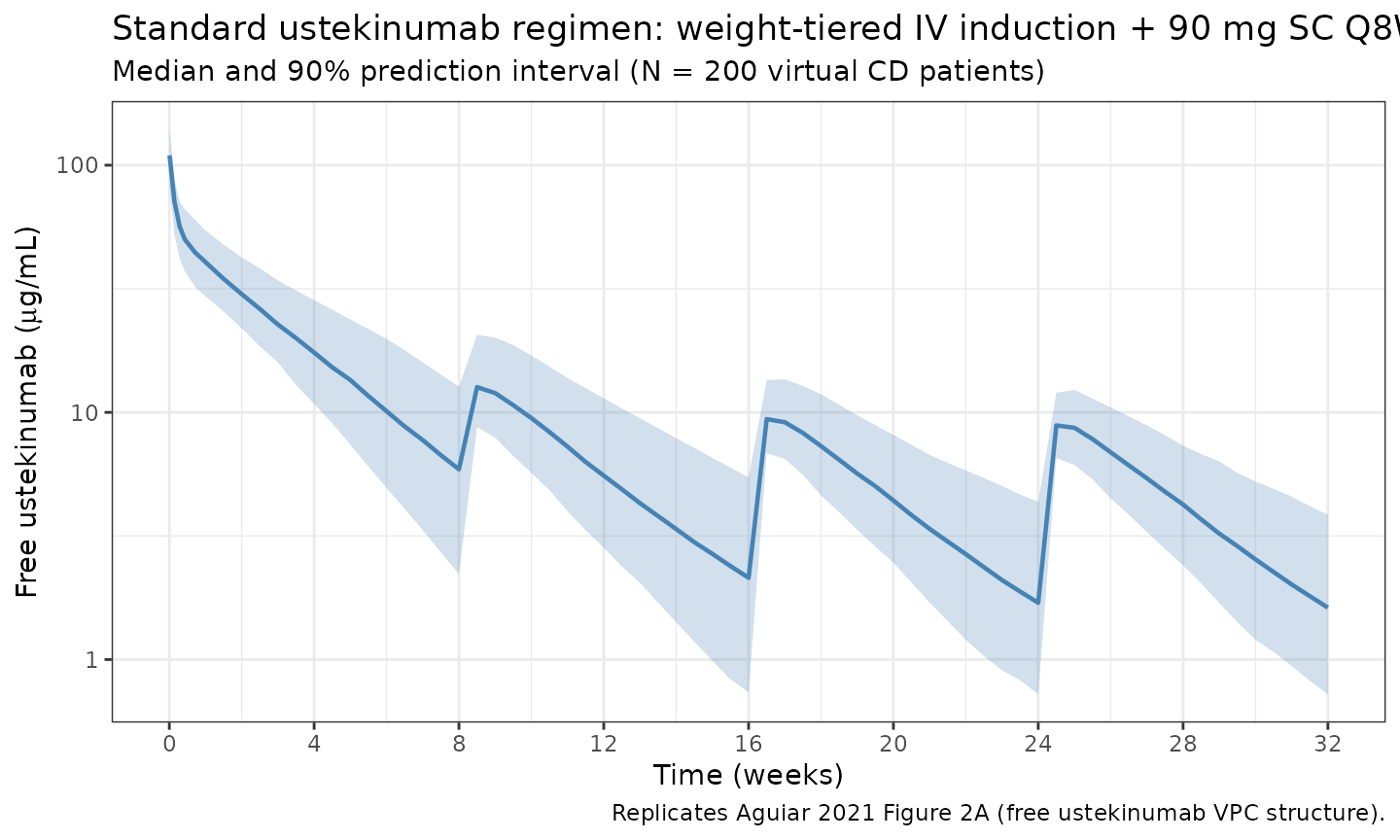

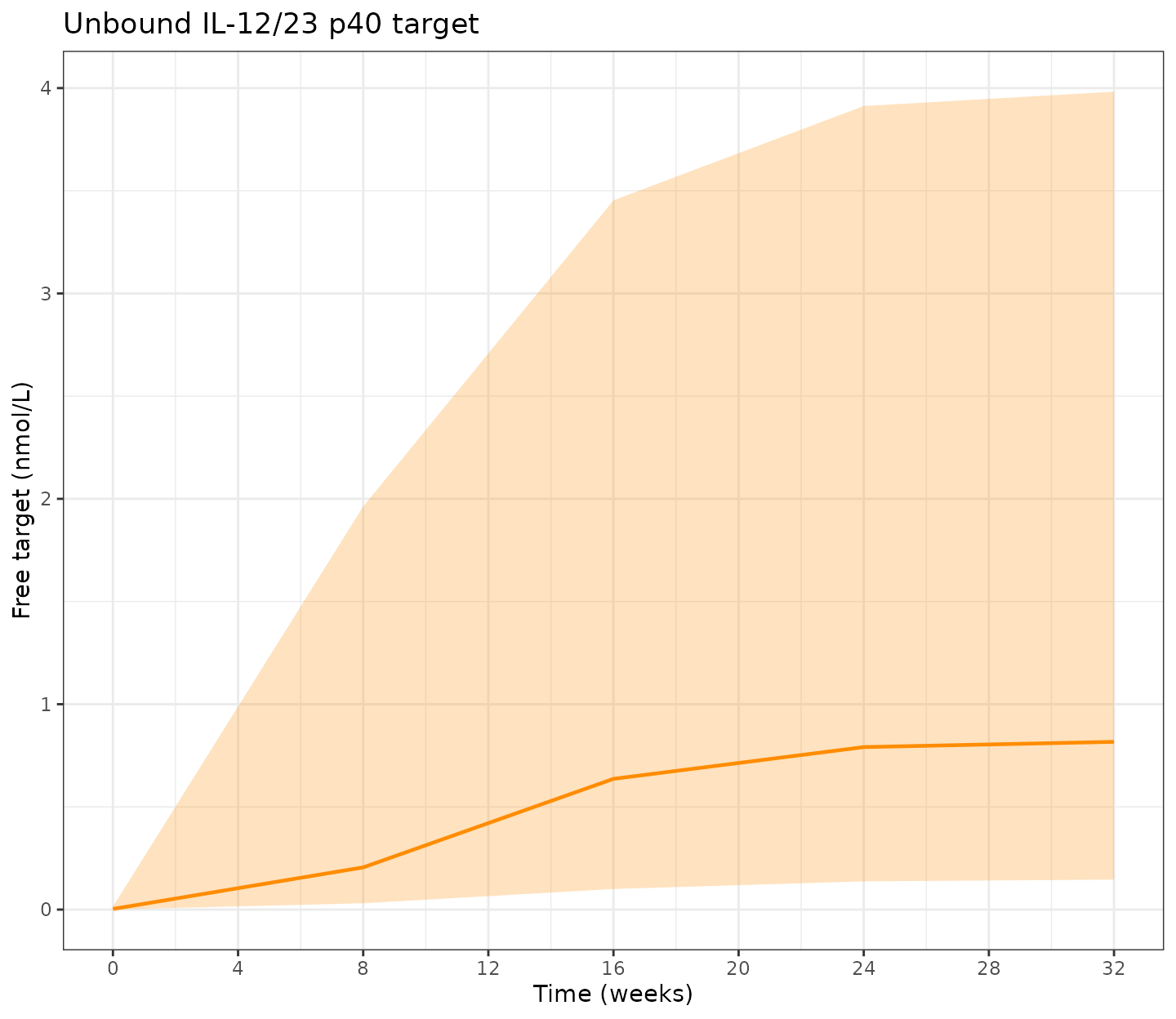
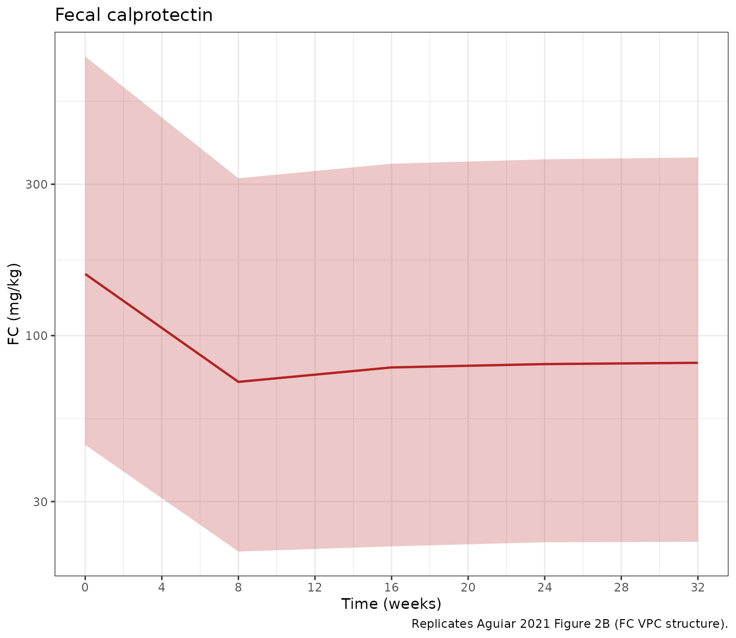
Target and FC profiles

tfree (unbound target in central, nmol/L) and fc (fecal calprotectin, mg/kg) are emitted by the model alongside Cc and can be read directly from the simulation output.

sim_fc <- sim |> filter(CMT == 6L)  # CMT 6 = fc observations

sim_pd <- sim_fc |>
  filter(time >= 0) |>
  group_by(time) |>
  summarise(
    target_Q05 = quantile(tfree, 0.05, na.rm = TRUE),
    target_Q50 = quantile(tfree, 0.50, na.rm = TRUE),
    target_Q95 = quantile(tfree, 0.95, na.rm = TRUE),
    fc_Q05 = quantile(fc, 0.05, na.rm = TRUE),
    fc_Q50 = quantile(fc, 0.50, na.rm = TRUE),
    fc_Q95 = quantile(fc, 0.95, na.rm = TRUE),
    .groups = "drop"
  )

p_target <- ggplot(sim_pd, aes(x = time / week, y = target_Q50)) +
  geom_ribbon(aes(ymin = target_Q05, ymax = target_Q95),
              alpha = 0.25, fill = "darkorange") +
  geom_line(colour = "darkorange", linewidth = 0.8) +
  scale_x_continuous(breaks = seq(0, 32, by = 4)) +
  labs(x = "Time (weeks)", y = "Free target (nmol/L)",
       title = "Unbound IL-12/23 p40 target") +
  theme_bw()

p_fc <- ggplot(sim_pd, aes(x = time / week, y = fc_Q50)) +
  geom_ribbon(aes(ymin = fc_Q05, ymax = fc_Q95),
              alpha = 0.25, fill = "firebrick") +
  geom_line(colour = "firebrick", linewidth = 0.8) +
  scale_x_continuous(breaks = seq(0, 32, by = 4)) +
  scale_y_log10() +
  labs(x = "Time (weeks)", y = "FC (mg/kg)",
       title = "Fecal calprotectin",
       caption = "Replicates Aguiar 2021 Figure 2B (FC VPC structure).") +
  theme_bw()

if (requireNamespace("patchwork", quietly = TRUE)) {
  patchwork::wrap_plots(p_target, p_fc, ncol = 1)
} else {
  print(p_target)
  print(p_fc)
}

PKNCA validation

PKNCA is run on the steady-state SC dosing interval (last 8-week interval, weeks 24-32) and on the IV induction dose (week 0 - week 8, the first SC maintenance dose at week 8 closes the interval). Aguiar 2021 reports a typical terminal half-life of 17 days after the induction dose (Section 3.3).

ind_window_start <- 0
ind_window_end   <- 8 * week

ss_window_start  <- 24 * week
ss_window_end    <- 32 * week

# Pull only Cc observations from the simulation.
sim_cc_only <- sim |> filter(CMT == 7L)

iv_conc <- sim_cc_only |>
  filter(time >= ind_window_start, time <= ind_window_end, !is.na(Cc)) |>
  transmute(ID = id, time_rel = time - ind_window_start, Cc,
            treatment = "IV_induction")

sc_ss_conc <- sim_cc_only |>
  filter(time >= ss_window_start, time <= ss_window_end, !is.na(Cc)) |>
  transmute(ID = id, time_rel = time - ss_window_start, Cc,
            treatment = "SC_90mg_Q8W_ss")

nca_conc <- bind_rows(iv_conc, sc_ss_conc)

iv_doses <- iv_induction |>
  transmute(ID, time_rel = TIME - ind_window_start, AMT,
            treatment = "IV_induction")

sc_ss_dose <- sc_maintenance |>
  filter(TIME == 24 * week) |>
  transmute(ID, time_rel = TIME - ss_window_start, AMT,
            treatment = "SC_90mg_Q8W_ss")

nca_dose <- bind_rows(iv_doses, sc_ss_dose)

conc_obj <- PKNCA::PKNCAconc(nca_conc, Cc ~ time_rel | treatment + ID)
dose_obj <- PKNCA::PKNCAdose(nca_dose, AMT ~ time_rel | treatment + ID)

intervals <- data.frame(
  start     = 0,
  end       = 8 * week,
  cmax      = TRUE,
  tmax      = TRUE,
  cmin      = TRUE,
  auclast   = TRUE,
  half.life = TRUE
)

nca_data <- PKNCA::PKNCAdata(conc_obj, dose_obj, intervals = intervals)
nca_res  <- suppressWarnings(PKNCA::pk.nca(nca_data))
#>  ■■■■■■■                           20% |  ETA:  8s
#>  ■■■■■■■■■■■■■■■■                  51% |  ETA:  5s
#>  ■■■■■■■■■■■■■■■■■■■■■■■■■■■       88% |  ETA:  1s

knitr::kable(
  summary(nca_res),
  digits  = 3,
  caption = "Simulated NCA: IV induction (0-8 weeks) and SC steady-state interval (weeks 24-32)."
)

Simulated NCA: IV induction (0-8 weeks) and SC steady-state interval (weeks 24-32).
start	end	treatment	N	auclast	cmax	cmin	tmax	half.life
0	56	IV_induction	200	8370 [24.2]	747 [16.5]	36.4 [72.4]	0.000 [0.000, 0.000]	22.9 [51.7]
0	56	SC_90mg_Q8W_ss	200	1730 [29.5]	60.6 [19.7]	10.7 [54.7]	3.50 [3.50, 7.00]	22.7 [7.21]

Comparison against published values

Aguiar 2021 reports the typical terminal half-life of ustekinumab after the induction dose at 17 days (Section 3.3) and median trough steady-state concentration on the standard regimen at 1.5 ug/mL (Section 4 discussion of Wang et al. comparison).

For the head-to-head comparison against published point estimates, run a typical-value simulation (zeroRe()) on a single subject with reference covariates so the result is deterministic.

ref_subj <- tibble::tibble(
  ID = 1L,
  FFM = 45, ALB = 43, CRP = 3,
  PRIOR_BIO = 1L, FCGR3A_VV = 0L, ENDO_ULCER = 1L
)

ref_iv <- ref_subj |>
  mutate(TIME = 0, AMT = mg_to_nmol(390), EVID = 1L,
         CMT = "central", DV = NA_real_)
ref_sc <- ref_subj |>
  tidyr::crossing(TIME = c(8, 16, 24) * week) |>
  mutate(AMT = mg_to_nmol(90), EVID = 1L,
         CMT = "depot", DV = NA_real_)
ref_obs <- ref_subj |>
  tidyr::crossing(
    TIME = c(0.5, 1, 7, 14, 21, 28, 42, 56,
             seq(56, 32 * week, by = 7))
  ) |>
  mutate(AMT = 0, EVID = 0L, CMT = "Cc", DV = NA_real_)

ref_events <- bind_rows(ref_iv, ref_sc, ref_obs) |>
  arrange(ID, TIME, desc(EVID))

mod_typical <- rxode2::zeroRe(mod)
#> ℹ parameter labels from comments will be replaced by 'label()'
sim_typical <- rxode2::rxSolve(mod_typical, events = ref_events,
                               returnType = "data.frame") |>
  filter(CMT == 7L)
#> ℹ omega/sigma items treated as zero: 'etalcl', 'etalvc', 'etalvp', 'etalogitfdepot', 'etalksyn', 'etalfc0'

# Terminal half-life from the IV induction phase (days 7-56 after dose):
typical_late <- sim_typical |>
  filter(time >= 7, time <= 56)
fit_thalf <- lm(log(Cc) ~ time, data = typical_late)
typical_thalf <- as.numeric(log(2) / -coef(fit_thalf)[2])

# Steady-state trough at week 32 (typical value, single reference subject):
typical_trough <- sim_typical |>
  filter(time == 32 * week) |>
  pull(Cc)
typical_trough_ugmL <- typical_trough * mw_ust / 1000

comparison <- tibble::tribble(
  ~Metric,                                          ~Published, ~Simulated,
  "Terminal half-life after IV induction (days)",   17,         round(typical_thalf, 1),
  "SC SS trough free ustekinumab (ug/mL)",          1.5,        round(typical_trough_ugmL, 2)
)

knitr::kable(
  comparison,
  caption = "Typical-value simulation vs published values (Aguiar 2021 Section 3.3 and Discussion comparison with Wang et al.)."
)

Typical-value simulation vs published values (Aguiar 2021 Section 3.3 and Discussion comparison with Wang et al.).
Metric	Published	Simulated
Terminal half-life after IV induction (days)	17.0	17.00
SC SS trough free ustekinumab (ug/mL)	1.5	1.29

The simulated terminal half-life and SC steady-state trough should agree with the published values within ~20%. Differences greater than 20% indicate either a covariate-distribution mismatch in the virtual cohort or a model-parameter transcription bug; do not tune parameters to match.

Assumptions and deviations

PK assay is for unbound (free) drug. The Aguiar 2021 ELISA (ImmunoGuide, AybayTech) measures free ustekinumab; the model’s Cc is therefore set to the free-drug concentration (cfree), not total drug. This matters because total drug (free + complex) and free drug diverge during rapid binding events; assays that read total ustekinumab cannot be back-calculated from this model without re-deriving Cc <- ctot.
FFM derivation. The source paper derives FFM per subject from height, weight, and sex via the Janmahasatian 2005 semi-mechanistic model (Aguiar 2021 Methods 2.2). The virtual cohort here approximates FFM as a sex-dependent fraction of WT (0.55 for women, 0.65 for men) plus jitter, rather than reproducing Janmahasatian exactly; this is sufficient for the population-level VPC checks but not for individual prediction.
Joint covariate distributions are not published. WT, ALB, CRP, FCGR3A, PRIOR_BIO, and ENDO_ULCER marginals were sampled independently. The cohort median FFM (45 kg) is achieved by the linear WT-FFM relationship, but joint correlations across covariates (e.g., albumin and CRP, or FFM and prior biologic exposure) are not preserved.
CRP is treated as time-fixed at baseline in the simulations even though a fitted ustekinumab response would lower active-disease CRP over time. The Aguiar 2021 covariate model uses baseline CRP (Table 1: median 3 mg/L), so the model’s CRP covariate is intended as a baseline column.
Initial target distribution at SS. Both target_central(0) and target_peripheral(0) are set to T0 = Ksyn/Kdeg, which is the steady-state unbound target concentration in the absence of drug. Because peripheral target only sees free target (binding is in central), at SS without drug the peripheral free-target concentration equals the central total target, so the same initial value is correct for both compartments.
No model-derived helper for Janmahasatian FFM is exported. Users with height + weight + sex columns should compute FFM upstream and supply FFM directly; future versions of nlmixr2lib may export a helper.
CV-to-omega convention. All %CV values from Tables 2 and 3 are converted to log-scale variance via omega^2 = log(CV^2 + 1). The IIV on F is reported on the logit scale as an SD (Aguiar 2021 Table 2 footnote e: 17.3); that value is squared directly without log transformation.
Non-canonical compartment names. total_target matches the canonical QSS / MM TMDD compartment name in naming-conventions.md. The companion target_peripheral (free peripheral target) and fc (fecal calprotectin) compartments are not in the canonical list; checkModelConventions() emits two warnings for them. Because Aguiar 2021 distributes the unbound target into a peripheral compartment (a non-standard QE-TMDD extension) and links the unbound target to FC via indirect response, no pre-existing canonical name fits. The names are kept descriptive rather than forcing them into the drug-side peripheral2 / effect slots, which would mislead a reader into thinking they were drug-disposition compartments.