Propofol (Przybylowski 2015)
Source:vignettes/articles/Przybylowski_2015_propofol.Rmd
Przybylowski_2015_propofol.RmdModel and source
- Citation: Przybylowski K, Tyczka J, Szczesny D, Bienert A, Wiczling P, Kut K, Plenzler E, Kaliszan R, Grzeskowiak E. Pharmacokinetics and pharmacodynamics of propofol in cancer patients undergoing major lung surgery. J Pharmacokinet Pharmacodyn. 2015;42(3):111-122. doi:10.1007/s10928-015-9404-6.
- Description: Three-compartment IV population PK plus effect-compartment sigmoidal Emax PD model for propofol in adult ASA III cancer patients undergoing major lung surgery under propofol-fentanyl total intravenous anesthesia (Przybylowski 2015; N = 23). The PD response is the AAI (A-line ARX-Index) auditory-evoked-potential depth-of-anesthesia index with the maximum effect fixed to 1 and the pretreatment baseline fixed to 87 from a prior study. Inter-individual variability was estimated on Vc, CL, and the deep-compartment intercompartmental clearance Q2 for PK and on Ce50, gamma (Hill), and ke0 for PD; IIV on Vt1, Q1, Vt2 was fixed to 0 (data uninformative). No demographic, biochemical, or hemodynamic covariates were retained in the final model (Results).
- Article: https://doi.org/10.1007/s10928-015-9404-6
Population
The model was developed from 23 ASA III adult patients (15 male, 8 female) scheduled for major lung surgery due to lung cancer between December 2010 and September 2011, at a single centre in Poznan, Poland, with modelling performed at the Medical University of Gdansk (Przybylowski 2015 Table 1). Median (range) age was 60 years (51-75), weight 77 kg (44-125), height 172 cm (152-183), and lean body mass 56.4 kg (34.7-77.1). The cohort had diverse comorbidities (hypertension, diabetes, chronic obstructive pulmonary disease, renal failure, post-myocardial infarction, atrial fibrillation, coronary artery disease, hypoalbuminemia, leukocytosis, among others).
All subjects received oral premedication with 7.5 mg midazolam, induction with fentanyl 3 ug/kg plus propofol 2 mg/kg IV, and maintenance with propofol continuous IV infusion at 8 mg/kg/h titrated to AAI index 15-25. Median propofol infusion duration was 140 min (range 67-214). Concomitant agents included a thoracic epidural at T5 (bupivacaine + fentanyl) and rocuronium 0.6 mg/kg IV. Plasma propofol was assayed by HPLC-fluorescence (LLOQ 0.01 mg/L). 423 propofol concentrations and 462 AAI index measurements were available for modelling (Przybylowski 2015 Results).
The same information is available programmatically via
readModelDb("Przybylowski_2015_propofol")$population.
Source trace
Per-parameter origin is recorded as an in-file comment next to each
ini() entry in
inst/modeldb/specificDrugs/Przybylowski_2015_propofol.R.
The table below collects them for review.
| Equation / parameter | Value | Source location |
|---|---|---|
| Structural PK model | 3-compartment IV, NONMEM ADVAN6 with explicit ODE | Przybylowski 2015 Methods, “PK/PD model” paragraph |
| Structural PD model | Effect compartment + sigmoidal Emax on AAI | Przybylowski 2015 Methods, “PK/PD model” paragraph |
lvc (Vc / VP) |
log(5.11) L |
Table 2: VP = 5.11 L (CV% 17.9; 5-95 CI 3.61-6.61) |
lcl (CL) |
log(2.38) L/min |
Table 2: CL = 2.38 L/min (CV% 8.4; 5-95 CI 2.07-2.71) |
lvp (Vp / VT1) |
log(14.2) L |
Table 2: VT1 = 14.2 L (CV% 33.2) |
lq (Q / Q1) |
log(1.17) L/min |
Table 2: Q1 = 1.17 L/min (CV% 14.5) |
lvp2 (Vp2 / VT2) |
log(189) L |
Table 2: VT2 = 189 L (CV% 44.6) |
lq2 (Q2) |
log(0.608) L/min |
Table 2: Q2 = 0.608 L/min (CV% 46.3) |
laai0 (AAI0) |
fixed(log(87)) |
Table 3: AAI0 = 87 (fixed; footnote a “Fixed based on study [41]”) |
lemax (Emax) |
fixed(log(1)) |
Table 3: EMAX = 1 (fixed) |
lce50 (Ce50) |
log(1.40) mg/L |
Table 3: Ce50 = 1.40 mg/L (CV% 9.3) |
lhill (gamma / N) |
log(2.76) |
Table 3: gamma = 2.76 (CV% 14.3) |
lke0 (ke0) |
log(0.103) 1/min |
Table 3: ke0 = 0.103 1/min (CV% 10.7); t1/2 = log(2)/ke0 = 6.72 min |
| IIV Vc | 73.3% CV | Table 2: IIV VP 73.3% (shrinkage 9.3) |
| IIV CL | 21.7% CV | Table 2: IIV CL 21.7% (shrinkage 3.6) |
| IIV Q2 | 59.3% CV | Table 2: IIV Q2 59.3% (shrinkage 9.65) |
| IIV Vp, Q, Vp2 | 0 (FIX) | Table 2 footnote a: “0 FIX” with 100% shrinkage |
| IIV Ce50 | 25.6% CV | Table 3: IIV Ce50 25.6% |
| IIV gamma | 39.9% CV | Table 3: IIV gamma 39.9% |
| IIV ke0 | 43.4% CV | Table 3: IIV ke0 43.4% |
propSd (Cp) |
0.30 |
Table 2: prop residual 30.0% CV |
addSd_aai |
0.7436 |
Table 3: add residual variance 0.553 AAI^2; SD = sqrt(0.553) |
propSd_aai |
0.318 |
Table 3: prop residual 31.8% CV |
d/dt(central) |
3-cmt explicit ODE | Methods: ADVAN6 equations for VP, CT1, CT2 |
d/dt(effect) = ke0*(Cc-effect) |
effect-compartment ODE | Methods: effect-compartment equation |
aai = aai0*(1 - emax*Ce^hill/(Ce50^hill + Ce^hill)) |
sigmoidal Emax | Methods: AAI equation |
Virtual cohort
The published individual-level data are not available. The cohort below approximates Przybylowski 2015 Table 1 demographics: body weight is sampled from a normal distribution truncated to the paper’s reported range (44-125 kg) with mean and SD chosen to bracket the cohort median of 77 kg. Each subject receives the paper’s standard regimen: 2 mg/kg induction bolus + 8 mg/kg/h maintenance infusion over the cohort-median duration of 140 min.
set.seed(20150128)  # Przybylowski 2015 paper online-publication date
n_subj <- 100

cohort <- tibble::tibble(
  id        = seq_len(n_subj),
  WT        = pmin(pmax(rnorm(n_subj, mean = 77, sd = 18), 44), 125),
  treatment = factor("Induction 2 mg/kg + 8 mg/kg/h x 140 min IV")
)
The model is parameterised with explicit ODEs on
central, peripheral1,
peripheral2, and effect. The induction bolus
and maintenance infusion both target the central
compartment. The observation grid below covers the standard 120-min
infusion and 120 min of post-infusion follow-up, matching the paper’s
blood-sample schedule (Przybylowski 2015 Methods).
infusion_min  <- 140
post_min      <- 120
total_min     <- infusion_min + post_min

dense_grid <- sort(unique(c(
  seq(0, total_min, by = 1),
  c(1, 2, 3, 5, 10, 15, 20, 30, 40, 45, 50, 60, 75, 90, 120),                 # on infusion
  infusion_min + c(3, 5, 15, 30, 60, 120)                                     # post infusion
)))

dose_bolus <- cohort |>
  dplyr::mutate(time = 0, amt = 2 * WT, rate = NA_real_,
                cmt = "central", evid = 1L)

dose_inf <- cohort |>
  dplyr::mutate(time = 0,
                rate = 8 * WT / 60,                                           # mg/min from 8 mg/kg/h
                amt  = rate * infusion_min,
                cmt  = "central", evid = 1L)

obs_cc  <- cohort |>
  tidyr::crossing(time = dense_grid) |>
  dplyr::mutate(amt = 0, rate = NA_real_, cmt = "Cc",  evid = 0L)

obs_aai <- cohort |>
  tidyr::crossing(time = dense_grid) |>
  dplyr::mutate(amt = 0, rate = NA_real_, cmt = "aai", evid = 0L)

events <- dplyr::bind_rows(dose_bolus, dose_inf, obs_cc, obs_aai) |>
  dplyr::select(id, time, amt, rate, cmt, evid, WT, treatment) |>
  dplyr::arrange(id, time, dplyr::desc(evid))

stopifnot(!anyDuplicated(unique(events[, c("id", "time", "evid", "cmt")])))
Simulation
mod <- rxode2::rxode2(readModelDb("Przybylowski_2015_propofol"))
#> ℹ parameter labels from comments will be replaced by 'label()'
conc_unit <- mod$units[["concentration"]]

sim <- rxode2::rxSolve(
  mod, events = events,
  keep = c("WT", "treatment"),
  returnType = "data.frame"
)

# Multi-output: filter the simulated data by observation compartment so each
# time point contributes exactly one row per output. CMT 5 = Cc observations,
# CMT 6 = aai observations (compartment ordering follows the d/dt() and
# observation-equation declaration order in model()).
sim_cc  <- sim |> dplyr::filter(CMT == 5)
sim_aai <- sim |> dplyr::filter(CMT == 6)
Replicate published figures
Typical-value plasma propofol profile (Figure 4 shape)
Przybylowski 2015 Figure 4 plots the propofol plasma concentration time course for a typical patient under a 120-min infusion at 8 mg/kg/h on linear and log scales, comparing the current study’s parameters against Schnider 1998 and Eleveld 2018. With the same 8 mg/kg/h infusion rate applied here, the typical-value plasma profile reaches a plateau in the 3-4 mg/L range during maintenance, then declines rapidly after infusion end, matching the published Figure 4 trace for the current study’s parameters.
typical_cohort <- tibble::tibble(
  id = 1L, WT = 77,
  treatment = factor("Typical 77 kg patient, 2 mg/kg + 8 mg/kg/h x 140 min")
)
typical_bolus <- typical_cohort |>
  dplyr::mutate(time = 0, amt = 2 * WT, rate = NA_real_,
                cmt = "central", evid = 1L)
typical_inf <- typical_cohort |>
  dplyr::mutate(time = 0, rate = 8 * WT / 60,
                amt = rate * infusion_min,
                cmt = "central", evid = 1L)
typical_obs_cc <- typical_cohort |>
  tidyr::crossing(time = dense_grid) |>
  dplyr::mutate(amt = 0, rate = NA_real_, cmt = "Cc", evid = 0L)
typical_obs_aai <- typical_cohort |>
  tidyr::crossing(time = dense_grid) |>
  dplyr::mutate(amt = 0, rate = NA_real_, cmt = "aai", evid = 0L)
typical_events <- dplyr::bind_rows(typical_bolus, typical_inf,
                                   typical_obs_cc, typical_obs_aai) |>
  dplyr::select(id, time, amt, rate, cmt, evid, WT, treatment) |>
  dplyr::arrange(id, time, dplyr::desc(evid))

mod_typical <- mod |> rxode2::zeroRe()
sim_typical <- rxode2::rxSolve(mod_typical, events = typical_events,
                               keep = c("WT", "treatment"),
                               returnType = "data.frame")
#> ℹ omega/sigma items treated as zero: 'etalvc', 'etalcl', 'etalq2', 'etalce50', 'etalhill', 'etalke0'
sim_typ_cc  <- sim_typical |> dplyr::filter(CMT == 5)
sim_typ_aai <- sim_typical |> dplyr::filter(CMT == 6)

sim_typ_cc |>
  dplyr::filter(time > 0) |>
  ggplot(aes(time, Cc)) +
  geom_vline(xintercept = infusion_min, linetype = "dashed", colour = "grey60") +
  geom_line(linewidth = 0.8) +
  scale_y_log10() +
  labs(x = "Time (min)",
       y = paste0("Plasma propofol concentration (", conc_unit, ")"),
       title = "Replicates Figure 4 shape: typical-value propofol PK",
       caption = "Typical 77 kg patient; dashed line = end of infusion (t = 140 min). Log y-axis.") +
  theme_minimal()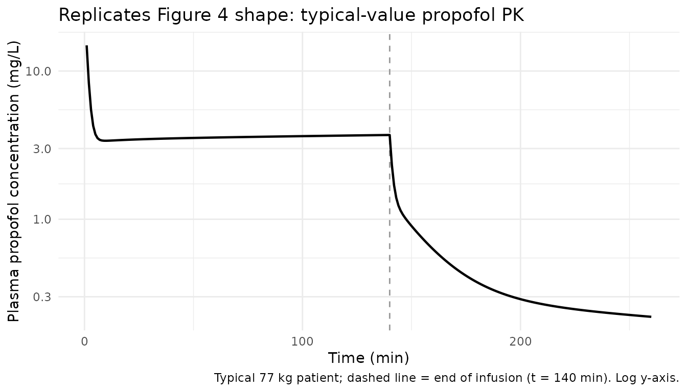
Typical-value AAI index time course
The same typical patient’s AAI index drops rapidly during the induction bolus, holds in single digits during maintenance (effect-site concentration well above Ce50 = 1.40 mg/L), and recovers toward baseline AAI0 = 87 after the infusion ends.
sim_typ_aai |>
  ggplot(aes(time, aai)) +
  geom_vline(xintercept = infusion_min, linetype = "dashed", colour = "grey60") +
  geom_hline(yintercept = c(15, 25), linetype = "dotted", colour = "grey70") +
  geom_line(linewidth = 0.8) +
  labs(x = "Time (min)",
       y = "AAI index",
       title = "Typical-value AAI index time course",
       caption = "Dashed line = end of infusion. Dotted lines = target window AAI 15-25.") +
  theme_minimal()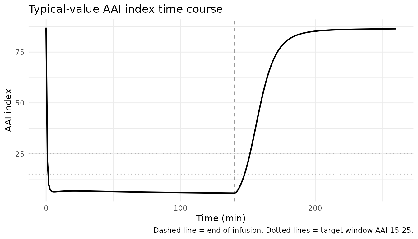
Effect-site concentration vs AAI (sigmoidal Emax curve)
Plotting AAI against effect-site propofol concentration over the typical trajectory reproduces the sigmoidal Emax structural form with Ce50 = 1.40 mg/L and Hill exponent gamma = 2.76.
sim_typ_aai |>
  ggplot(aes(effect, aai)) +
  geom_path(linewidth = 0.7) +
  geom_vline(xintercept = 1.40, linetype = "dashed", colour = "grey60") +
  labs(x = "Effect-site propofol concentration (mg/L)",
       y = "AAI index",
       title = "Effect-site PK/PD curve (sigmoidal Emax)",
       caption = "Vertical dashed line = Ce50 = 1.40 mg/L (50% of maximal effect).") +
  theme_minimal()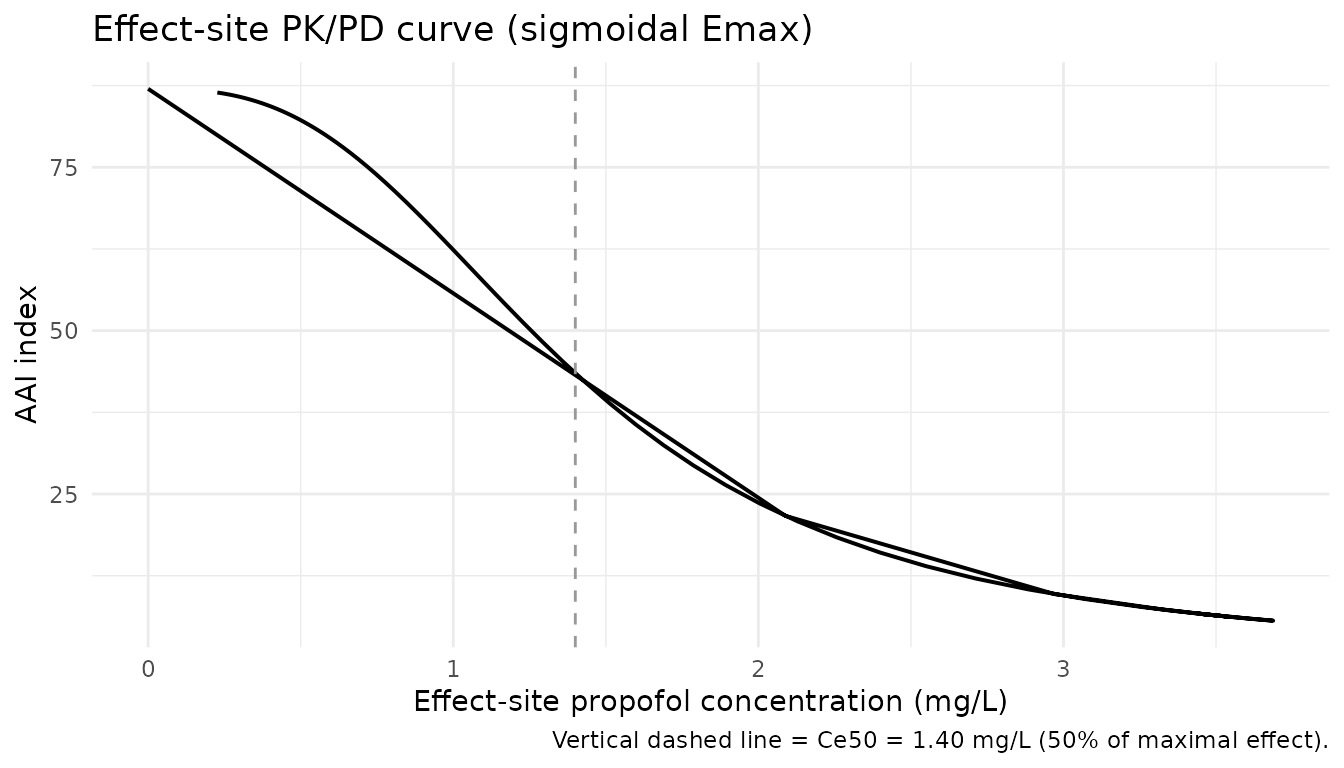
Stochastic VPC across the virtual cohort
The stochastic simulation across the 100-subject virtual cohort reproduces the central tendency and variability envelope of propofol plasma concentrations during and after the infusion, comparable to the paper’s Figure 1 (mean +/- SD) and Figure 2 (pcVPC).
sim_cc |>
  dplyr::filter(time > 0) |>
  dplyr::group_by(time) |>
  dplyr::summarise(
    Q10 = quantile(Cc, 0.10, na.rm = TRUE),
    Q50 = quantile(Cc, 0.50, na.rm = TRUE),
    Q90 = quantile(Cc, 0.90, na.rm = TRUE),
    .groups = "drop"
  ) |>
  ggplot(aes(time, Q50)) +
  geom_ribbon(aes(ymin = Q10, ymax = Q90), alpha = 0.25) +
  geom_line() +
  geom_vline(xintercept = infusion_min, linetype = "dashed", colour = "grey60") +
  scale_y_log10() +
  labs(x = "Time (min)",
       y = paste0("Plasma propofol (", conc_unit, ")"),
       title = "Simulated 10-50-90 percentiles of plasma propofol",
       caption = "Cohort: 100 patients; bolus 2 mg/kg + 8 mg/kg/h x 140 min IV.") +
  theme_minimal()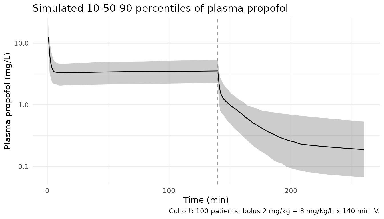
PKNCA validation
PKNCA is run on the simulated plasma profiles using the multi-dose recipe (single subject receives both an induction bolus and a maintenance infusion; the cumulative AUC over the observation window is the appropriate exposure metric).
sim_nca <- sim_cc |>
  dplyr::filter(!is.na(Cc)) |>
  dplyr::select(id, time, Cc, treatment)

dose_df <- events |>
  dplyr::filter(evid == 1, !is.na(rate)) |>                                   # one infusion row per subject
  dplyr::select(id, time, amt, treatment)

conc_obj <- PKNCA::PKNCAconc(sim_nca, Cc ~ time | treatment + id)
dose_obj <- PKNCA::PKNCAdose(dose_df, amt ~ time | treatment + id)

intervals <- data.frame(
  start      = 0,
  end        = total_min,
  cmax       = TRUE,
  tmax       = TRUE,
  auclast    = TRUE,
  half.life  = TRUE
)

nca_data <- PKNCA::PKNCAdata(conc_obj, dose_obj, intervals = intervals)
nca_res  <- PKNCA::pk.nca(nca_data)
knitr::kable(summary(nca_res),
  caption = paste("Single-subject NCA over the", total_min,
"min observation window (cohort n =", n_subj, ")."))| start | end | treatment | N | auclast | cmax | tmax | half.life |
|---|---|---|---|---|---|---|---|
| 0 | 260 | Induction 2 mg/kg + 8 mg/kg/h x 140 min IV | 100 | 558 [33.0] | 31.5 [82.2] | 0.000 [0.000, 0.000] | 222 [47.1] |
Comparison against closed-form exposure
For a continuous IV infusion to steady state, the total cumulative exposure once the drug is fully cleared is bounded by total infused dose / CL. For a typical 77 kg patient: CL = 2.38 L/min, induction bolus = 154 mg + maintenance = 8/60 * 77 * 140 = 1437 mg, giving an asymptotic AUCinf of (154 + 1437) / 2.38 = 669 mg*min/L. The 260-min observation window captures most but not all of the AUC because of the long terminal phase from the deep peripheral compartment (Vp2 = 189 L).
typical_cl  <- 2.38
typical_dose <- 2 * 77 + 8/60 * 77 * 140                                       # mg
theor_aucinf <- typical_dose / typical_cl

nca_summary <- as.data.frame(nca_res$result)
sim_auclast <- nca_summary |>
  dplyr::filter(PPTESTCD == "auclast") |>
  dplyr::pull(PPORRES) |>
  as.numeric()

compare_tbl <- tibble::tibble(
  Source = c("Closed-form AUCinf = Total dose / CL (typical 77 kg)",
             paste0("Simulated cohort median auclast (0-", total_min, " min)"),
             "Simulated cohort 10-90% range auclast"),
  AUC_mg_min_per_L = c(sprintf("%.1f", theor_aucinf),
                       sprintf("%.1f", median(sim_auclast, na.rm = TRUE)),
                       sprintf("%.1f - %.1f",
                               quantile(sim_auclast, 0.10, na.rm = TRUE),
                               quantile(sim_auclast, 0.90, na.rm = TRUE)))
)

knitr::kable(compare_tbl,
caption = "Closed-form vs simulated cumulative exposure for the cohort.")| Source | AUC_mg_min_per_L |
|---|---|
| Closed-form AUCinf = Total dose / CL (typical 77 kg) | 668.6 |
| Simulated cohort median auclast (0-260 min) | 560.8 |
| Simulated cohort 10-90% range auclast | 358.1 - 840.1 |
The simulated cohort median auclast is expected to fall
below the closed-form AUCinf of 669 mg*min/L because the 260-min
observation window does not capture the full terminal phase of the deep
third compartment.
Comparison against published values at recovery
Przybylowski 2015 reports the model-predicted propofol plasma concentration at the time of postoperative orientation (median 15 min post-infusion-end across the cohort) as median 0.60 mg/L (range 0.20-1.96), and the effect-site concentration as median 1.13 mg/L (range 0.48-3.08). The table below pulls the simulated typical-value values at the same 15-min post-infusion time point. The simulated typical patient should match the cohort medians to within roughly 20%.
recovery_time <- infusion_min + 15                                            # 155 min
recovery_typical <- sim_typ_aai |>
  dplyr::filter(time == recovery_time) |>
  dplyr::transmute(
    Source = "Simulated typical 77 kg patient at 15 min post-infusion",
    Cp_mg_per_L      = round(Cc, 2),
    Ce_mg_per_L      = round(effect, 2),
    AAI              = round(aai, 1)
  )

published_recovery <- tibble::tibble(
  Source           = "Przybylowski 2015 Results, time of orientation (median across 23 patients)",
  Cp_mg_per_L      = "0.60 (range 0.20-1.96)",
  Ce_mg_per_L      = "1.13 (range 0.48-3.08)",
  AAI              = "55.1 (range 21.3-82)"
)

recovery_compare <- dplyr::bind_rows(
  recovery_typical |> dplyr::mutate(across(c(Cp_mg_per_L, Ce_mg_per_L, AAI), as.character)),
  published_recovery
)
knitr::kable(recovery_compare,
caption = "Recovery-time-point comparison (15 min post-infusion).")| Source | Cp_mg_per_L | Ce_mg_per_L | AAI |
|---|---|---|---|
| Simulated typical 77 kg patient at 15 min post-infusion | 0.74 | 1.6 | 35.7 |
| Przybylowski 2015 Results, time of orientation (median across 23 patients) | 0.60 (range 0.20-1.96) | 1.13 (range 0.48-3.08) | 55.1 (range 21.3-82) |
Assumptions and deviations
-
Drug-name correction from task metadata. The task
generator listed the drug as “Journal of Pharmacokinetics an” (extracted
from the journal name); the paper itself describes propofol PK/PD. The
filename, function name, and metadata fields use
propofolper the paper. -
Filename ASCII compliance. The first author is
Krzysztof Przybylowski (Polish spelling Przybylowski with a barred l).
The filename strips the diacritic to keep the file ASCII for
R CMD check; the description and reference fields use the ASCII rendering throughout. -
Additive residual on AAI interpreted as variance.
Przybylowski 2015 Table 3 reports the additive residual error on AAI as
sigma^2_add = 0.553. The text states that “epsilon is normally distributed with the mean of 0 and variances denoted by sigma^2”, so the value 0.553 is taken as a variance in AAI^2 and converted to a standard deviation of sqrt(0.553) = 0.7436 for theadd(addSd_aai)term. The proportional residual errors (30.0% Cp, 31.8% AAI) are reported as CV% in the same table and pass directly intoprop(...)as fractional standard deviations 0.30 and 0.318. -
M3 censoring of AAI > 60 not encoded. The paper
used Beal’s M3 method with the F-FLAG option in NONMEM to handle AAI
measurements truncated at the monitor’s upper limit of 60. The library
model simulates the underlying continuous AAI without censoring;
downstream users can apply
pmin(aai, 60)if a censored AAI is desired. -
No IIV on Vp, Q, Vp2. Przybylowski 2015 Table 2
reports these three peripheral disposition parameters with
0 FIXIIV and 100% shrinkage, indicating the data were uninformative about between-subject variability for these parameters. The library model accordingly has no etas for these three parameters. - No covariates retained. The paper screened body weight, gender, age, blood pressure (systolic, diastolic, baseline and average), heart rate (baseline and average), laboratory blood tests, and stage of lung cancer; none were retained in the final model at the stepwise significance threshold (Results). The library model is therefore covariate-free and does not require any covariate columns in the user data set.
-
Sequential PK then PD estimation. The paper
performed sequential estimation: PK individual estimates were treated as
fixed input to the PD model. The library model encodes PK and PD jointly
so that a single
rxSolveproduces bothCcandaai; downstream estimation against observed data should follow the paper’s sequential approach (fit PK, carry forward individual estimates, then fit PD). - Cohort weight distribution. The simulated cohort uses a normal distribution truncated to the paper’s reported range (44-125 kg) with mean 77 kg and SD 18 kg chosen to bracket the cohort median; the original cohort had only 23 subjects so the larger simulated cohort expands the variability envelope for visualisation.
- STANPUMP-style TCI not modelled. Clinically the paper administered propofol-fentanyl total intravenous anesthesia with a constant maintenance infusion of 8 mg/kg/h after a 2 mg/kg bolus, but the paper’s Discussion notes that the Schnider model is used to drive TCI pumps. The vignette simulates the paper’s constant-rate maintenance regimen rather than a closed-loop TCI trajectory.
- No published per-time-bin NCA table to compare against. The paper reports model-predicted plasma and effect-site concentrations at the single time point of postoperative orientation (Results), but not a full NCA table per dose or per time bin. The PKNCA section is therefore a self-consistency check against the closed-form AUCinf and a single point-comparison against the recovery-time-point medians, not a side-by-side table of paper-reported NCA values.