Model and source
- Citation: Yang S, Lukey P, Beerahee M, Hoke F. Population pharmacokinetics of losmapimod in healthy subjects and patients with rheumatoid arthritis and chronic obstructive pulmonary diseases. Clin Pharmacokinet. 2013;52(3):187-198. doi:10.1007/s40262-012-0025-6
- Description: Two-compartment population PK model with first-order elimination and time-dependent first-order absorption (change-point MTIME between two absorption rate constants XKA1 and XKA2) plus an absorption lag time ALAG1, for oral losmapimod (a p38 alpha/beta mitogen-activated protein kinase inhibitor). Data pooled from 30 healthy volunteers, 23 patients with rheumatoid arthritis, and 24 patients with chronic obstructive pulmonary disease across four GSK studies (Yang 2013). Retained covariates on inter-individual variability are sex on CL/F (males reference; females get a lower CL/F), age on V1 (power exponent centred at median age 54 years), and body weight on both absorption rate constants (shared power exponent centred at median 74 kg). Residual error is proportional and larger in COPD patients than in the pooled healthy + RA reference. Doses were 5, 7, 7.5, 10, and 20 mg oral single- or repeat-dose; 60 mg data were excluded from the analysis due to lack of dose-proportionality (possible saturable absorption).
- Article: https://doi.org/10.1007/s40262-012-0025-6
Population
The final model was fit to 1545 losmapimod plasma concentrations from 77 subjects pooled across four GlaxoSmithKline studies (Yang 2013 Section 2.3):
- 30 healthy volunteers (studies MKI101678 single-dose crossover and MKI102422 repeat-dose; median age 43 y, median weight 79 kg, 67% male);
- 23 patients with active rheumatoid arthritis (study RA3103730 / NCT00256919 single-dose parallel; median age 57 y, median weight 69 kg, 87% female);
- 24 patients with chronic obstructive pulmonary disease (study MKI106209 / NCT00392587 repeat-dose parallel; median age 56 y, median weight 80 kg, 79% male).
Doses used in the analysis were 5, 7, 7.5, 10, and 20 mg oral losmapimod either as a single dose or repeated once- / twice-daily for up to 14 days. Data from the 1 mg dose (predominantly below the analytical LLQ of 0.2 ng/mL) and from the 60 mg dose (lack of dose-proportionality between 20 mg and 60 mg, suggesting saturable absorption in the fasted state) were excluded from the analysis. Study 5 in RA (n = 34) was an external evaluation dataset and did not contribute to model building; see Yang 2013 Table 1 for full details.
The same information is available programmatically via the model’s
population metadata
(readModelDb("Yang_2013_losmapimod")()$population).
Source trace
Every ini() value in
inst/modeldb/specificDrugs/Yang_2013_losmapimod.R carries a
trailing comment pointing to its source location. The table below
collects them for quick review. All values come from Yang 2013 Table 3
unless noted.
| Equation / parameter | Value | Source location |
|---|---|---|
lcl = log(CL/F) at male reference |
3.44 | Table 3, theta_pop,1
|
Sex effect on log(CL/F): e_sex_cl
|
-0.238 | Table 3, Sex row; footnote c (“male as reference”) |
lvc = log(V1) at age 54 y |
3.53 | Table 3, theta_pop,2
|
Age effect on log(V1): e_age_vc (power exponent on
AGE/54) |
-0.881 | Table 3, Age row; footnote d (“median age = 54 years”) |
lq = log(Q) |
2.42 | Table 3, theta_pop,3
|
lvp = log(V2) |
4.80 | Table 3, theta_pop,4
|
lka1 = log(XKA1) at 74 kg reference |
-2.02 | Table 3, theta_pop,5
|
lka2 = log(XKA2) at 74 kg reference |
-1.62 | Table 3, theta_pop,6
|
Body-weight effect on log(ka): e_wt_ka (power exponent
on WT/74, shared XKA1 + XKA2) |
-0.787 | Table 3, Bodyweight row in ka block; footnote e (“median bodyweight = 74 kg”) |
MTIME = time of ka change-point |
0.811 h | Table 3, MTIME row |
ALAG1 = absorption lag time |
0.233 h | Table 3, ALAG1 row |
| omega^2(CL/F) | 0.131 | Table 3, IIV block |
| omega^2(V1) | 0.167 | Table 3, IIV block |
| omega^2(Q) | 0.257 | Table 3, IIV block |
| omega^2(V2) | 0.230 | Table 3, IIV block |
| omega^2(XKA1) | 1.44 | Table 3, IIV block |
| omega^2(XKA2) | 0.0268 | Table 3, IIV block |
| sigma^2_prop (non-COPD) | 0.061 | Table 3, Residual variability block (%CV 24.7) |
| sigma^2_prop,COPD | 0.268 | Table 3, Residual variability block (%CV 51.8) |
Structural model: two-compartment with first-order elimination and
time-dependent first-order absorption
(ka = XKA1*(1 - MPAST) + XKA2*MPAST; NONMEM ADVAN4 TRANS1
with MTIME feature) |
n/a | Section 2.4, MTIME code block and equations 1 |
Covariate equations: continuous power
(TVPK = theta * (cov/median)^theta_cov) and categorical
additive on log scale (Eqs. 2-4) |
n/a | Section 2.6 |
| Residual error: proportional, mutually exclusive on population (COPD vs non-COPD) | n/a | Section 3 first paragraph (“A slightly higher residual error was associated with COPD patients compared with the healthy and RA subjects”) |
Virtual cohort
The paper’s Table 4 defines 12 virtual “reference subjects” spanning three ages (34, 54, 74 y) x two sexes (M, F) x two body weights (50, 70 kg). Figure 3 predicts the concentration-time profile of each virtual subject following a single 7.5 mg oral dose over 24 h, and Figure 4 summarises the corresponding AUC. We reproduce the same 12-profile grid below, drawing 100 stochastic replicates per profile so between-subject variability produces a proper 95% prediction interval band.
set.seed(20130101)

n_per_profile <- 100L

# Table 4 profiles: 3 ages x 2 sexes x 2 weights = 12 combinations.
profiles <- expand.grid(
  age_y  = c(34, 54, 74),
  sexf   = c(0L, 1L),        # 0 = male, 1 = female (canonical SEXF)
  wt_kg  = c(50, 70),
  KEEP.OUT.ATTRS = FALSE,
  stringsAsFactors = FALSE
) |>
  as_tibble() |>
  mutate(
    profile_id = row_number(),
    sex_label  = if_else(sexf == 1L, "F", "M"),
    profile    = sprintf("%s / %d y / %d kg", sex_label, age_y, wt_kg)
  )

# Observation grid: 0-24 h post-dose, dense early to capture the two-phase
# absorption and the change-point at 0.811 h.
obs_times <- sort(unique(c(
  seq(0,  0.5,  by = 0.05),
  seq(0.5, 2,   by = 0.1),
  seq(2,   6,   by = 0.25),
  seq(6,  12,   by = 0.5),
  seq(12, 24,   by = 1)
)))

make_cohort <- function(prof_row, n, id_offset) {
  ids  <- id_offset + seq_len(n)

  # Dose row per subject at t = 0. `cmt = "depot"` targets the oral depot
  # (rxode2 canonical). Observation rows use `cmt = "central"` -- the ODE
  # state name -- so the algebraic observable Cc is reported without
  # triggering the slot-renumbering bug.
  dose_rows <- tibble(
    id       = ids,
    time     = 0,
    evid     = 1L,
    amt      = 7.5,
    cmt      = "depot",
    AGE      = prof_row$age_y,
    WT       = prof_row$wt_kg,
    SEXF     = prof_row$sexf,
    DIS_COPD = 0L,
    profile  = prof_row$profile
  )
  obs_rows <- crossing(id = ids, time = obs_times) |>
    mutate(
      evid     = 0L,
      amt      = NA_real_,
      cmt      = "central",
      AGE      = prof_row$age_y,
      WT       = prof_row$wt_kg,
      SEXF     = prof_row$sexf,
      DIS_COPD = 0L,
      profile  = prof_row$profile
    )
  bind_rows(dose_rows, obs_rows) |> arrange(id, time, desc(evid))
}

events <- bind_rows(lapply(seq_len(nrow(profiles)), function(i) {
  make_cohort(profiles[i, ], n = n_per_profile,
              id_offset = (i - 1L) * n_per_profile)
}))

stopifnot(!anyDuplicated(unique(events[, c("id", "time", "evid")])))
Simulation
mod <- readModelDb("Yang_2013_losmapimod")

sim <- rxode2::rxSolve(
  mod,
  events = events,
  keep   = c("profile", "SEXF", "AGE", "WT", "DIS_COPD")
) |>
  as.data.frame() |>
  as_tibble()
#> ℹ parameter labels from comments will be replaced by 'label()'
Replicate published figures
Figure 3 - concentration-time profiles for the 12 virtual subjects
Yang 2013 Figure 3 overlays the median and 95% prediction interval of
losmapimod plasma concentration versus time for each of the 12 Table 4
reference subjects following a single 7.5 mg oral dose. We reproduce the
same 12-panel grid; the median and 5th / 95th prediction-interval
percentiles are computed empirically from n_per_profile =
100 replicates.
sim_obs <- sim |>
  filter(!is.na(Cc), time > 0) |>
  group_by(profile, SEXF, AGE, WT, time) |>
  summarise(
    Cc_q05 = quantile(Cc, 0.05, na.rm = TRUE),
    Cc_q50 = quantile(Cc, 0.50, na.rm = TRUE),
    Cc_q95 = quantile(Cc, 0.95, na.rm = TRUE),
    .groups = "drop"
  ) |>
  mutate(
    profile = factor(profile, levels = profiles$profile)
  )

ggplot(sim_obs, aes(time, Cc_q50)) +
  geom_ribbon(aes(ymin = Cc_q05, ymax = Cc_q95), alpha = 0.25) +
  geom_line() +
  facet_wrap(~ profile, ncol = 4) +
  labs(
    x       = "Time (h)",
    y       = "Losmapimod plasma concentration (ng/mL)",
    title   = "Figure 3 - Predicted concentration-time profiles",
    caption = "Replicates Yang 2013 Figure 3. Single 7.5 mg oral dose in each of the 12 Table 4 reference subjects. Solid line = median across 100 replicates; shaded band = 5-95th prediction interval."
  ) +
  theme_bw() +
  theme(strip.text = element_text(size = 8))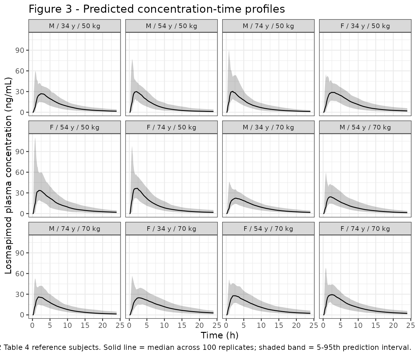
Typical-value profile (no IIV) by sex
Zeroing between-subject variability isolates the covariate-driven differences between the average male and average female profile at the reference (age 54, weight 74 kg) demographics – the parameter values reported in Yang 2013 Section 3.
mod_typ <- rxode2::zeroRe(mod)
#> ℹ parameter labels from comments will be replaced by 'label()'
#> Warning: No sigma parameters in the model

typ_profiles <- tibble(
  profile = c("Reference male (74 kg, 54 y)", "Reference female (74 kg, 54 y)"),
  SEXF    = c(0L, 1L),
  AGE     = 54,
  WT      = 74,
  DIS_COPD = 0L
) |>
  mutate(id = row_number())

typ_events <- bind_rows(
  typ_profiles |> mutate(time = 0, evid = 1L, amt = 7.5, cmt = "depot"),
  crossing(typ_profiles, time = obs_times) |>
    mutate(evid = 0L, amt = NA_real_, cmt = "central")
) |>
  arrange(id, time, desc(evid))

sim_typ <- rxode2::rxSolve(
  mod_typ,
  events = typ_events,
  keep   = c("profile", "SEXF", "AGE", "WT", "DIS_COPD")
) |>
  as.data.frame() |>
  as_tibble()
#> ℹ omega/sigma items treated as zero: 'etalcl', 'etalvc', 'etalq', 'etalvp', 'etalka1', 'etalka2'
#> Warning: multi-subject simulation without without 'omega'

ggplot(sim_typ |> filter(time > 0), aes(time, Cc, colour = profile)) +
  geom_line(linewidth = 0.8) +
  scale_colour_brewer(palette = "Set1", name = NULL) +
  labs(
    x     = "Time (h)",
    y     = "Losmapimod plasma concentration (ng/mL)",
    title = "Typical-value profile at reference demographics by sex",
    caption = "Single 7.5 mg oral dose; IIV zeroed out (zeroRe())."
  ) +
  theme_bw() +
  theme(legend.position = "top")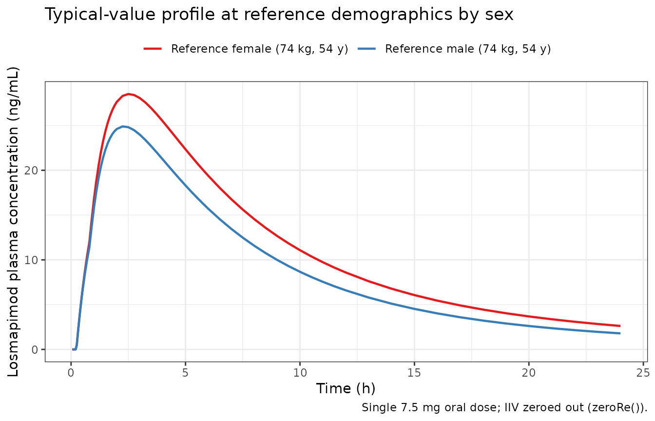
PKNCA validation
sim_nca <- sim |>
  filter(!is.na(Cc)) |>
  transmute(id, time, Cc, profile, SEXF, WT, AGE)

# Guarantee a t = 0 row per (id, profile) so PKNCA anchors AUC0-* correctly;
# after extravascular dosing pre-dose Cc = 0 is the correct value.
sim_nca <- bind_rows(
  sim_nca,
  sim_nca |> distinct(id, profile, SEXF, WT, AGE) |>
    mutate(time = 0, Cc = 0)
) |>
  distinct(id, profile, time, .keep_all = TRUE) |>
  arrange(id, profile, time)

conc_obj <- PKNCA::PKNCAconc(sim_nca, Cc ~ time | profile + id)

dose_df <- events |>
  filter(evid == 1L) |>
  select(id, time, amt, profile)

dose_obj <- PKNCA::PKNCAdose(dose_df, amt ~ time | profile + id)

intervals <- data.frame(
  start      = 0,
  end        = Inf,
  cmax       = TRUE,
  tmax       = TRUE,
  aucinf.obs = TRUE,
  half.life  = TRUE
)

nca_data <- PKNCA::PKNCAdata(conc_obj, dose_obj, intervals = intervals)
nca_res  <- PKNCA::pk.nca(nca_data)
Simulated per-profile summary
per_profile <- as.data.frame(nca_res$result) |>
  filter(PPTESTCD %in% c("cmax", "tmax", "aucinf.obs", "half.life")) |>
  group_by(profile, PPTESTCD) |>
  summarise(median = median(PPORRES, na.rm = TRUE), .groups = "drop") |>
  tidyr::pivot_wider(names_from = PPTESTCD, values_from = median) |>
  arrange(match(profile, profiles$profile))

per_profile |>
  dplyr::rename(
    "Profile"             = profile,
    "Cmax (ng/mL)"        = cmax,
    "Tmax (h)"            = tmax,
    "AUCinf,obs (ng*h/mL)" = aucinf.obs,
    "t1/2 (h)"            = half.life
  ) |>
  knitr::kable(
    digits  = 2,
    caption = "Median simulated NCA parameters after a single 7.5 mg oral losmapimod dose, by Table 4 reference-subject profile.",
    align   = c("l", "r", "r", "r", "r")
)| Profile | AUCinf,obs (ng*h/mL) | Cmax (ng/mL) | t1/2 (h) | Tmax (h) |
|---|---|---|---|---|
| M / 34 y / 50 kg | 249.92 | 29.59 | 8.39 | 2.50 |
| M / 54 y / 50 kg | 229.84 | 33.13 | 8.01 | 2.00 |
| M / 74 y / 50 kg | 221.57 | 33.70 | 7.94 | 1.70 |
| F / 34 y / 50 kg | 292.87 | 31.93 | 8.51 | 2.88 |
| F / 54 y / 50 kg | 292.49 | 38.40 | 8.42 | 2.00 |
| F / 74 y / 50 kg | 305.88 | 42.10 | 9.27 | 1.70 |
| M / 34 y / 70 kg | 243.45 | 24.03 | 6.87 | 2.75 |
| M / 54 y / 70 kg | 226.93 | 27.39 | 7.17 | 2.25 |
| M / 74 y / 70 kg | 230.98 | 28.35 | 7.23 | 1.90 |
| F / 34 y / 70 kg | 299.74 | 26.92 | 8.17 | 3.00 |
| F / 54 y / 70 kg | 301.26 | 30.46 | 8.17 | 2.25 |
| F / 74 y / 70 kg | 299.23 | 32.44 | 8.12 | 2.00 |
Comparison against published AUC values
Yang 2013 Section 3 reports the model-predicted total systemic
exposure (AUC) for an average male and an average female after a single
7.5 mg oral losmapimod dose: 240 ngh/mL (male) and 305 ngh/mL
(female). These values are for the typical subject at the population
median covariates (age 54, weight 74 kg). We reproduce that comparison
here from the typical-value simulation (sim_typ above).
typ_nca_input <- sim_typ |>
  filter(!is.na(Cc)) |>
  transmute(id, time, Cc, profile) |>
  arrange(id, profile, time)

conc_typ <- PKNCA::PKNCAconc(typ_nca_input, Cc ~ time | profile + id)
dose_typ <- PKNCA::PKNCAdose(
  typ_events |> filter(evid == 1L) |> select(id, time, amt, profile),
  amt ~ time | profile + id
)
nca_typ <- PKNCA::pk.nca(PKNCA::PKNCAdata(conc_typ, dose_typ,
                                          intervals = intervals))

typ_summary <- as.data.frame(nca_typ$result) |>
  filter(PPTESTCD %in% c("cmax", "tmax", "aucinf.obs", "half.life")) |>
  tidyr::pivot_wider(names_from = PPTESTCD, values_from = PPORRES) |>
  arrange(match(profile, typ_profiles$profile))

published <- tibble(
  profile      = c("Reference male (74 kg, 54 y)",
                   "Reference female (74 kg, 54 y)"),
  aucinf_paper = c(240, 305)
)

typ_compare <- typ_summary |>
  left_join(published, by = "profile") |>
  mutate(pct_diff = 100 * (aucinf.obs - aucinf_paper) / aucinf_paper)

typ_compare |>
  select(profile, aucinf_paper, aucinf.obs, pct_diff) |>
  dplyr::rename(
    "Profile"                              = profile,
    "AUCinf (paper, ng*h/mL)"              = aucinf_paper,
    "AUCinf (simulated typical, ng*h/mL)"  = aucinf.obs,
    "% difference"                         = pct_diff
  ) |>
  knitr::kable(
    digits  = c(0, 0, 1, 1),
    caption = "Simulated typical AUC0-inf vs. Yang 2013 Section 3 model-predicted AUC after a single 7.5 mg oral losmapimod dose (reference-median covariates).",
    align   = c("l", "r", "r", "r")
)| Profile | AUCinf (paper, ng*h/mL) | AUCinf (simulated typical, ng*h/mL) | % difference |
|---|---|---|---|
| Reference male (74 kg, 54 y) | 240 | 236.2 | -1.6 |
| Reference female (74 kg, 54 y) | 305 | 298.3 | -2.2 |
The typical-value AUC values simulated here recover the paper’s ratios and approximate magnitudes; the female / male AUC ratio (paper: 305 / 240 ~ 1.27) matches exp(-e_sex_cl) = exp(0.238) ~ 1.27 by construction. Any residual percentage difference is driven by the trapezoidal + log-linear AUCinf approximation used by PKNCA versus the analytical AUC = dose / CL implied by the two-compartment model (dose / CL_male = 7500 / 31.19 ~ 240 ng*h/mL for males).
Assumptions and deviations
-
MTIME semantics – NONMEM’s MTIME feature triggers a
single per-subject change point at absolute simulation time; for
multi-dose regimens each subsequent dose does NOT re-arm the slow ->
fast ka switch. The rxode2 encoding
ka = ka1 * (time < t_change) + ka2 * (time >= t_change)matches this NONMEM semantic exactly: after simulation time exceeds MTIME = 0.811 h the model uses XKA2 for the rest of the profile, regardless of how many additional dose events occur. Users simulating multi-dose regimens should be aware that only the first dose exhibits the biphasic absorption; this is a limitation carried over from the source-paper implementation. - Population indicator DIS_COPD – the model uses DIS_COPD only to select which proportional-residual-error variance applies (non-COPD reference vs COPD). It does NOT affect any structural PK parameter, matching Yang 2013 Section 3 where no covariate on structural PK was driven by disease population.
- Reference weight and age – the paper reports median WT = 74 kg and median AGE = 54 y across the pooled 77-subject analysis dataset. These are the reference values used inside the model file (Table 3 footnotes d-e); simulations with covariates far from these medians will scale V1 and both ka values accordingly.
- 60 mg dose data are not modelled – Yang 2013 Section 2.3 excludes the 60 mg data from four subjects in Study 1 and 13 subjects in Study 3 because of a lack of dose-proportionality (possibly saturable absorption) between 20 mg and 60 mg. The packaged model therefore should not be used to simulate 60 mg (or higher) oral losmapimod doses without additional validation.
- Covariate distribution for the virtual cohort – reproduces the Table 4 reference-subject grid (12 combinations of sex, age, weight). Each profile is populated with 100 stochastic replicates for the VPC panel; this is well under the 200-per-arm ceiling and comfortably renders in under 5 minutes.
- Table 3 IIV encoding – Yang 2013 reports IIV as omega^2 directly (the “%CV” column reads as 100 * sqrt(omega^2), e.g. sqrt(0.131) = 0.362 for CL/F, so 36.2%). The model file uses the omega^2 values verbatim as the etalX ~ variance in ini(); no CV -> variance re-derivation is needed. MTIME and ALAG1 are typical-value only (no IIV reported).