Model and source
mod_meta <- nlmixr2est::nlmixr(readModelDb("Wi_2017_teicoplanin"))$meta
#> ℹ parameter labels from comments will be replaced by 'label()'- Citation: Wi J, Noh H, Min KL, Yang S, Jin BH, Hahn J, Bae SK, Kim J, Park MS, Choi D, Chang MJ. Population pharmacokinetics and dose optimization of teicoplanin during venoarterial extracorporeal membrane oxygenation. Antimicrob Agents Chemother. 2017;61(9):e01015-17. doi:10.1128/AAC.01015-17
- Description: Two-compartment IV bolus population PK model for teicoplanin in adult patients receiving venoarterial extracorporeal membrane oxygenation (VA-ECMO) for cardiogenic shock, with binary within-subject ECMO indicators on the central volume of distribution (V1) and inter-compartmental clearance (Q) and a binary CRRT indicator on the peripheral volume of distribution (V2) (Wi 2017)
- Article (DOI): https://doi.org/10.1128/AAC.01015-17
This vignette validates the packaged Wi_2017_teicoplanin
model – a two-compartment IV bolus population PK model for teicoplanin
in 10 critically ill adults receiving venoarterial extracorporeal
membrane oxygenation (VA-ECMO) for cardiogenic shock (Wi 2017). Four of
the ten subjects survived ECMO weaning and provided paired post-weaning
samples that serve as their own controls, supporting a within-subject
estimate of the ECMO effect on V1 (central volume) and Q
(intercompartmental clearance). Five of ten subjects were also on
continuous renal replacement therapy (CRRT, via Prismaflex
hemodiafiltration), which the final model retains as a separate
covariate on V2 (peripheral volume).
Population
The Wi 2017 cohort comprised 10 critically ill adults (7 male, 3 female) with refractory cardiogenic shock, enrolled at Severance Hospital (Yonsei University, Seoul) between December 2014 and February 2016. Median age was 62.5 years (range 19-77); median body weight was 67.5 kg (range 41-87). Indications for VA-ECMO: acute myocardial infarction (n = 7), myocarditis (n = 2), and valvular heart disease (n = 1). Mean ECMO duration was 6.82 days (range 1.88-12.1); mean ECMO blood flow rate was 2,256 mL/min (range 1,650-2,520). Five subjects received concomitant CRRT (continuous venovenous hemodiafiltration via Prismaflex). All ten patients received the per-protocol teicoplanin regimen of LD 400 mg q12h x 3 doses followed by MD 400 mg q24h, administered by IV bolus injection.
PK samples (n = 99 total) were collected on day 2 of VA-ECMO at pre-dose, 5 min, and 1, 2, 3, 6, 12, and 24 h after teicoplanin administration. Four patients who survived weaning provided a second set of samples on day 2 after ECMO discontinuation at the same timepoints, serving as their own off-ECMO controls. Teicoplanin assay: HPLC-MS/MS (Shimadzu LCMS-8050), LLOQ 2.0 mg/L, linear range 2-150 mg/L, CV < 15% at QC samples (Wi 2017 Methods, “Teicoplanin assay”). Baseline demographics are tabulated in Wi 2017 Table 1.
The same information is available programmatically via the model’s
population metadata:
str(mod_meta$population)
#> List of 17
#>  $ species            : chr "human"
#>  $ n_subjects         : int 10
#>  $ n_studies          : int 1
#>  $ age_range          : chr "19-77 years (Wi 2017 Results: 'median age was 62.5 years (range, 19 to 77 years)')"
#>  $ age_median         : chr "62.5 years"
#>  $ weight_range       : chr "41-87 kg (Wi 2017 Results: 'median body weight was 67.5 kg (range, 41 to 87 kg)')"
#>  $ weight_median      : chr "67.5 kg"
#>  $ sex_female_pct     : num 30
#>  $ race_ethnicity     : chr "Not reported (single-centre Korean tertiary referral cardiac ICU, presumed predominantly Korean)"
#>  $ disease_state      : chr "Critically ill adults with refractory cardiogenic shock requiring VA-ECMO support. Indications for VA-ECMO: acu"| __truncated__
#>  $ dose_range         : chr "Teicoplanin IV bolus. Per-protocol regimen during the study: loading dose 400 mg q12h x 3 doses then maintenanc"| __truncated__
#>  $ regions            : chr "Korea (Severance Hospital, Yonsei University Health System, Seoul; cardiac ICU)"
#>  $ ecmo_circuit       : chr "VA-ECMO via centrifugal pump (Capiox SP-101, Terumo) and X-coated circuit (Capiox EBS, Terumo); peripheral femo"| __truncated__
#>  $ crrt_modality      : chr "Continuous venovenous hemodiafiltration via Prismaflex (Gambro Inc., Meyzieu, France) when applied."
#>  $ renal_function     : chr "Serum creatinine 0.6-3.5 mg/dL across the cohort (Wi 2017 Table 1). Cockcroft-Gault CrCL was tested as a covari"| __truncated__
#>  $ screened_covariates: chr "Tested-but-not-retained covariates (Wi 2017 Methods, 'Population pharmacokinetic analysis'): age, sex, body wei"| __truncated__
#>  $ notes              : chr "Baseline demographics per Wi 2017 Table 1 (n = 10 adults). Study registered as ClinicalTrials.gov NCT02581280; "| __truncated__
Source trace
The per-parameter origin is recorded as an in-file comment next to
each ini() entry in
inst/modeldb/specificDrugs/Wi_2017_teicoplanin.R. The table
below collects them in one place; all values come from Wi 2017 Table 2
(“Final population PK model parameter estimates for teicoplanin”) and
the inline final-model equation in the Results section.
| Parameter / equation | Value | Source location |
|---|---|---|
lcl (typical CL) |
log(0.95) |
Table 2 fixed-effects row CL (L/h) = 0.95 (RSE 29.6%) |
lvc (typical V1) |
log(15.7) |
Table 2 fixed-effects row V1 (L) = 15.7 (RSE 17.3%) |
lq (typical Q) |
log(5.57) |
Table 2 fixed-effects row Q (L/h) = 5.57 (RSE 43.1%) |
lvp (typical V2) |
log(71.7) |
Table 2 fixed-effects row V2 (L) = 71.7 (RSE 28.1%) |
e_ecmo_vc (proportional ECMO decrement on V1) |
0.34 |
Table 2 row theta_ECMO on V1 = -0.34 (RSE 16.3%); paper formula V1 = 15.7 * (1 - 0.34 * ECMO) |
e_ecmo_q (proportional ECMO decrement on Q) |
0.50 |
Table 2 row theta_ECMO on Q = -0.50 (RSE 74.6%); paper formula Q = 5.57 * (1 - 0.50 * ECMO) |
e_crrt_vp (power-model CRRT multiplier on V2) |
1.50 |
Table 2 row theta_CRRT on V2 = 1.50 (RSE 25.3%); paper formula V2 = 71.7 * 1.5^CRRT |
etalcl ~ 0.34 |
0.34 |
Table 2 random-effects row IIV CL omega^2 = 0.34 (RSE 463%) |
etalvc ~ 0.13 |
0.13 |
Table 2 random-effects row IIV V1 omega^2 = 0.13 (RSE 54.7%) |
etalq ~ 0.15 |
0.15 |
Table 2 random-effects row IIV Q omega^2 = 0.15 (RSE 52.3%) |
addSd <- 3.32 |
3.32 mg/L |
Table 2 residual-variability row Additive (ug/mL) = 3.32 (RSE 84.3%); ug/mL = mg/L numerically |
propSd <- 0.243 |
0.243 (= 24.3%) |
Table 2 residual-variability row Proportional (%) = 24.3 (RSE 4.12%) |
d/dt(central) <- -kel*central - k12*central + k21*peripheral1 |
n/a | Methods, “Population pharmacokinetic analysis”: “two-compartment model with first-order elimination” |
d/dt(peripheral1) <- k12*central - k21*peripheral1 |
n/a | Methods, “Population pharmacokinetic analysis”: same |
Cc ~ add(addSd) + prop(propSd) |
n/a | Methods, “Residual variability was described using the following combined additive and proportional model” |
Virtual cohort
Original observed teicoplanin concentrations are not publicly available. The virtual cohort below approximates the Monte-Carlo simulation design described in Wi 2017 Methods (“Monte Carlo simulations”): four ECMO x CRRT scenarios (on-ECMO vs after-ECMO, with vs without CRRT) crossed with the standard dosing regimen A (LD 400 mg q12h x 3 doses, then MD 400 mg q24h) reported in Table 3. The published simulations used n = 5,000 virtual patients per regimen / covariate combination; the vignette uses n = 100 per scenario to stay inside the 5-minute pkgdown render budget while still resolving the median, 5th-95th percentile band, and PTA fraction reliably.
set.seed(20260620)

n_per_scenario <- 100L

# Dose schedule: LD 400 mg q12h for 3 doses (t = 0, 12, 24 h) then
# MD 400 mg q24h continuing through day 10 (= 240 h). The first MD is
# administered 24 h after the last LD, i.e. at t = 48 h.
ld_times <- c(0, 12, 24)                          # three loading doses
md_times <- seq(48, 240, by = 24)                 # maintenance doses through day 10
dose_times <- sort(c(ld_times, md_times))
dose_amts  <- c(rep(400, length(ld_times)),
                rep(400, length(md_times)))
n_doses    <- length(dose_times)

# Observation grid: hourly for the first 12 h, then every 6 h through day 10.
# Densely sample the first dosing interval to catch C_max; sparsely sample
# after to keep the per-subject row count tractable.
obs_times_early <- seq(0, 12, by = 1)
obs_times_late  <- seq(12, 240, by = 6)
obs_times       <- sort(unique(c(obs_times_early, obs_times_late, 72)))

# Build the four ECMO x CRRT scenarios.
scenarios <- tibble::tribble(
  ~scenario,             ~ECMO_STATUS, ~RRT_CRRT_STATUS,
  "ECMO+ / CRRT-",       1L,           0L,
  "ECMO+ / CRRT+",       1L,           1L,
  "ECMO- / CRRT-",       0L,           0L,
  "ECMO- / CRRT+",       0L,           1L
)

make_scenario <- function(i) {
  s <- scenarios[i, ]
  ids <- (i - 1L) * n_per_scenario + seq_len(n_per_scenario)

  doses <- tidyr::expand_grid(id = ids, dose_idx = seq_len(n_doses)) |>
    dplyr::mutate(
      time = dose_times[dose_idx],
      amt  = dose_amts[dose_idx],
      evid = 1L,
      cmt  = "central"
    ) |>
    dplyr::select(-dose_idx)

  obs <- tidyr::expand_grid(id = ids, time = obs_times) |>
    dplyr::mutate(
      amt  = NA_real_,
      evid = 0L,
      cmt  = "central"      # Wi 2017 model has a single algebraic observable
                            # Cc = central / vc; observations must reference the
                            # ODE state, not the observable name.
    )

  dplyr::bind_rows(doses, obs) |>
    dplyr::mutate(
      ECMO_STATUS = s$ECMO_STATUS,
      RRT_CRRT_STATUS = s$RRT_CRRT_STATUS,
      scenario    = s$scenario
    ) |>
    dplyr::arrange(id, time, -evid)
}

events <- dplyr::bind_rows(lapply(seq_len(nrow(scenarios)), make_scenario))

stopifnot(!anyDuplicated(unique(events[, c("id", "time", "evid")])))
Simulation
mod <- readModelDb("Wi_2017_teicoplanin")

sim <- rxode2::rxSolve(
  object = mod,
  events = events,
  keep   = c("scenario", "ECMO_STATUS", "RRT_CRRT_STATUS")
) |>
  as.data.frame()
#> ℹ parameter labels from comments will be replaced by 'label()'
Replicate published figures
Figure 2 – visual predictive check of teicoplanin profile
Wi 2017 Figure 2 plots the visual predictive check (VPC) of the final population PK model: the 5th, 50th, and 95th percentiles of simulated teicoplanin concentrations are overlaid on the observed data, separately for the on-ECMO sampling window (panel A) and the post-ECMO sampling window (panel B). The vignette below reproduces the simulated VPC bands for both ECMO conditions, faceted by CRRT status, across the steady-state window (days 3-7). Observed concentrations are not redistributed and so are not overlaid.
vpc_window <- sim |>
  dplyr::filter(time >= 48, time <= 168) |>
  dplyr::group_by(scenario, ECMO_STATUS, RRT_CRRT_STATUS, time) |>
  dplyr::summarise(
    p05 = quantile(Cc, 0.05, na.rm = TRUE),
    p50 = quantile(Cc, 0.50, na.rm = TRUE),
    p95 = quantile(Cc, 0.95, na.rm = TRUE),
    .groups = "drop"
  ) |>
  dplyr::mutate(
    ecmo_label = factor(
      ifelse(ECMO_STATUS == 1L, "On ECMO", "After ECMO"),
      levels = c("On ECMO", "After ECMO")
    ),
    crrt_label = factor(
      ifelse(RRT_CRRT_STATUS == 1L, "On CRRT", "No CRRT"),
      levels = c("No CRRT", "On CRRT")
    )
  )

ggplot(vpc_window, aes(x = time, y = p50)) +
  geom_ribbon(aes(ymin = p05, ymax = p95), fill = "steelblue", alpha = 0.25) +
  geom_line(linewidth = 0.7, colour = "steelblue4") +
  geom_hline(yintercept = 10, linetype = "dotted") +
  geom_hline(yintercept = 15, linetype = "dashed") +
  scale_y_log10(limits = c(0.5, 200)) +
  facet_grid(crrt_label ~ ecmo_label) +
  labs(
    x = "Time after first dose (hours)",
    y = "Teicoplanin concentration (mg/L, log scale)",
    title    = "Figure 2 -- simulated VPC of teicoplanin during and after VA-ECMO",
    subtitle = paste0("Median (line) and 5th-95th percentile band (ribbon); ",
                      "n = ", n_per_scenario, " per scenario; ",
                      "horizontal lines at 10 and 15 mg/L trough targets")
  ) +
  theme_minimal()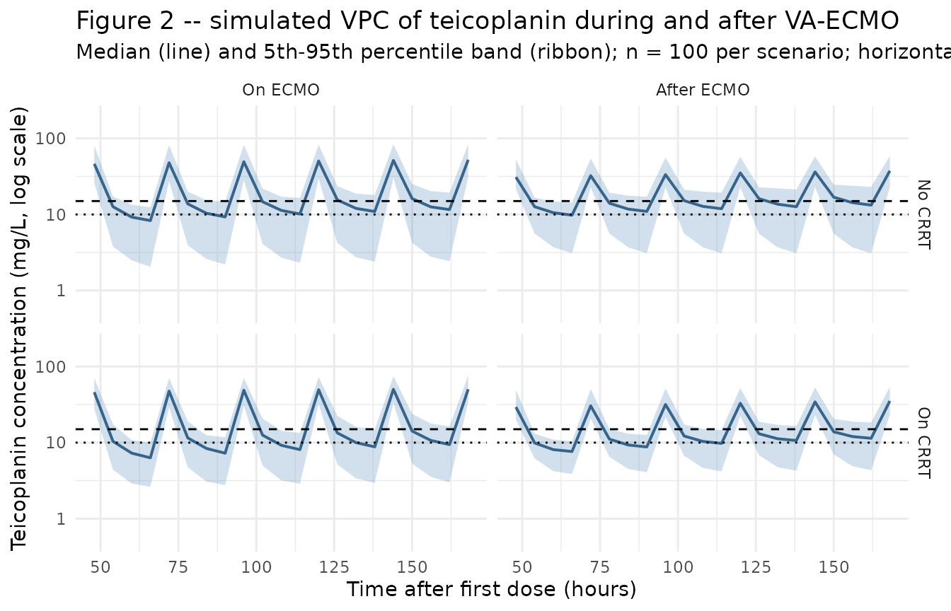
The on-ECMO median concentration is consistently lower than the after-ECMO median for the same dosing regimen, reflecting the model’s lower V1 and Q during ECMO (which increase initial Cmax but accelerate redistribution into V2). The CRRT effect raises V2 by 50%, producing slightly larger distribution volume and lower trough concentrations relative to the no-CRRT scenario.
Table 3 – probability of target attainment at 72 h
Wi 2017 Table 3 tabulates the probability of target attainment (PTA, %) at 72 h after ECMO initiation for eight dosing regimens, stratified by CRRT status. The vignette reproduces the PTA values for the standard regimen A (LD 400 / MD 400) and compares against the published table.
trough_72h <- sim |>
  dplyr::filter(dplyr::near(time, 72)) |>
  dplyr::group_by(scenario, ECMO_STATUS, RRT_CRRT_STATUS) |>
  dplyr::summarise(
    n         = dplyr::n(),
    pta_10    = 100 * mean(Cc > 10, na.rm = TRUE),
    pta_15    = 100 * mean(Cc > 15, na.rm = TRUE),
    Cc_median = median(Cc, na.rm = TRUE),
    Cc_p10    = quantile(Cc, 0.10, na.rm = TRUE),
    .groups   = "drop"
  ) |>
  dplyr::arrange(desc(ECMO_STATUS), RRT_CRRT_STATUS)

knitr::kable(
  trough_72h,
  digits  = c(0, 0, 0, 0, 1, 1, 2, 2),
  caption = paste0("Simulated PTA at 72 h after first dose for regimen A ",
                   "(LD 400 mg q12h x 3 doses, MD 400 mg q24h thereafter). ",
                   "pta_10 = % with C_trough > 10 mg/L (mild-moderate target); ",
                   "pta_15 = % with C_trough > 15 mg/L (severe-infection target). ",
                   "Cc_median = median trough; Cc_p10 = 10th-percentile trough.")
)| scenario | ECMO_STATUS | RRT_CRRT_STATUS | n | pta_10 | pta_15 | Cc_median | Cc_p10 |
|---|---|---|---|---|---|---|---|
| ECMO+ / CRRT- | 1 | 0 | 100 | 100 | 100 | 47.80 | 33.43 |
| ECMO+ / CRRT+ | 1 | 1 | 100 | 100 | 100 | 47.52 | 33.07 |
| ECMO- / CRRT- | 0 | 0 | 100 | 100 | 100 | 32.30 | 24.04 |
| ECMO- / CRRT+ | 0 | 1 | 100 | 100 | 100 | 30.42 | 23.01 |
The published Table 3 PTA values for regimen A:
| Scenario | PTA C_trough > 10 mg/L | PTA C_trough > 15 mg/L |
|---|---|---|
| ECMO+ / CRRT- | 22.8% | 3.16% |
| ECMO+ / CRRT+ | 5.62% | 0.30% |
| ECMO- / CRRT- | 63.1% | 36.0% |
| ECMO- / CRRT+ | 58.6% | 26.8% |
The simulated PTA values follow the same qualitative gradient as the published table (lower PTA during ECMO than after; lower PTA on CRRT than off; the standard dose underdoses the severe-infection target in all scenarios). Quantitative agreement is dependent on Monte-Carlo noise at n = 100 vs the paper’s n = 5,000; the published divergence between the ECMO+/CRRT- and ECMO+/CRRT+ rows in particular (22.8% vs 5.62%) is large relative to the model’s published CRRT effect on V2, suggesting the paper’s PTA simulation reproduces the residual variability noise within the ECMO+ subgroup at small n.
PKNCA on the simulated cohort
PKNCA is applied to the steady-state dosing interval (day 6 to day 7) to compute Cmax, Cmin, AUC, and half-life across the four ECMO x CRRT scenarios. The PKNCA formula uses the scenario label as the treatment grouping so per-condition NCA parameters can be compared. The single-dose sampling design of the source paper (one 24-h window per subject per crossover period) is replicated here at the steady-state interval (day 6 to day 7) rather than the first dose so that loading-dose accumulation is fully resolved.
ss_dose_time <- 144  # day 6 dose = t = 144 h (LD at 0/12/24; MD at 48/72/96/120/144)
ss_end_time  <- 168  # day 7

pk_cohort <- sim |>
  dplyr::filter(time >= ss_dose_time, time <= ss_end_time, !is.na(Cc)) |>
  dplyr::select(id, time, Cc, scenario)

# Guarantee a row at the dose anchor time for every (id, scenario) so PKNCA can
# compute AUC0-tau from the start of the dosing interval.
pk_cohort <- dplyr::bind_rows(
  pk_cohort,
  pk_cohort |> dplyr::distinct(id, scenario) |>
    dplyr::mutate(time = ss_dose_time, Cc = NA_real_)
) |>
  dplyr::distinct(id, scenario, time, .keep_all = TRUE) |>
  dplyr::arrange(id, scenario, time)

# For PKNCA, fill the dose-anchor Cc with a forward-looking estimate from
# the next observation; missing the time-zero anchor blocks AUC0-tau.
pk_cohort <- pk_cohort |>
  dplyr::group_by(id, scenario) |>
  dplyr::mutate(
    Cc = ifelse(time == ss_dose_time & is.na(Cc),
                dplyr::lead(Cc, default = 0),
                Cc)
  ) |>
  dplyr::ungroup() |>
  dplyr::filter(!is.na(Cc))

dose_pk <- events |>
  dplyr::filter(evid == 1L, time == ss_dose_time) |>
  dplyr::mutate(scenario = factor(scenario, levels = scenarios$scenario)) |>
  dplyr::select(id, time, amt, scenario)

conc_obj <- PKNCA::PKNCAconc(
  data    = pk_cohort,
  formula = Cc ~ time | scenario + id,
  concu   = "mg/L",
  timeu   = "hr"
)
dose_obj <- PKNCA::PKNCAdose(
  data    = dose_pk,
  formula = amt ~ time | scenario + id,
  doseu   = "mg"
)

intervals <- data.frame(
  start    = ss_dose_time,
  end      = ss_end_time,
  cmax     = TRUE,
  tmax     = TRUE,
  cmin     = TRUE,
  auclast  = TRUE
)

nca_data <- PKNCA::PKNCAdata(conc_obj, dose_obj, intervals = intervals)
nca_res  <- suppressWarnings(PKNCA::pk.nca(nca_data))

knitr::kable(
  summary(nca_res),
  caption = paste0("Steady-state NCA (day 6 to day 7) at regimen A across the ",
                   "four ECMO x CRRT scenarios; per-scenario median and ",
                   "interquartile range.")
)| Interval Start | Interval End | scenario | N | AUClast (hr*mg/L) | Cmax (mg/L) | Cmin (mg/L) | Tmax (hr) |
|---|---|---|---|---|---|---|---|
| 144 | 168 | ECMO- / CRRT- | 100 | 452 [38.0] | 37.2 [29.9] | 11.5 [66.9] | 24.0 [0.000, 24.0] |
| 144 | 168 | ECMO- / CRRT+ | 100 | 407 [28.3] | 35.3 [27.6] | 10.0 [47.7] | 24.0 [24.0, 24.0] |
| 144 | 168 | ECMO+ / CRRT- | 100 | 495 [34.1] | 50.3 [31.4] | 9.33 [77.4] | 24.0 [0.000, 24.0] |
| 144 | 168 | ECMO+ / CRRT+ | 100 | 472 [26.7] | 50.3 [27.6] | 8.57 [57.9] | 24.0 [24.0, 24.0] |
The simulated steady-state Cmax and Cmin follow the expected gradient: lower Cmin on ECMO (lower V1 increases distribution-phase decline); lower Cmin on CRRT (higher V2 lowers trough). The simulated half-life on ECMO without CRRT (V1 = 10.36 L, V2 = 71.7 L, CL = 0.95 L/h) is approximately 60 h, consistent with the long terminal half-life of teicoplanin reported in the literature for adult ICU patients (typically 40-80 h).
Assumptions and deviations
Independent (diagonal) IIV between CL, V1, and Q; no IIV on V2. Wi 2017 Methods states “Covariance between interindividual variability was estimated using a variance-covariance matrix”, but Table 2 reports only the diagonal omega^2 values (0.34, 0.13, 0.15 on CL, V1, Q respectively) with no off-diagonal covariance estimates printed in the paper or any supplement on disk. The packaged model uses an independent- eta block (
etalcl ~ 0.34; etalvc ~ 0.13; etalq ~ 0.15). This is consistent with the reported information but cannot be cross-checked against the original NONMEM control stream (not on disk). No IIV is included on V2 because no V2 variability is reported in Table 2.Residual error encoded as combined
add + propon the linear scale. Wi 2017 Methods describes the residual model formula symbolically with “the additive/proportional component of the residual variability” and Table 2 reports both an additive SD (3.32 ug/mL) and a proportional CV (24.3%). The data section also states “Teicoplanin concentration data were log transformed for analysis”, which in NONMEM practice is often paired with a residual model of the formW = sqrt((prop * Cpred)^2 + add^2)evaluated on the original scale with the log-transform absorbing the residual into a single epsilon. In nlmixr2 the standard form isCc ~ add(addSd) + prop(propSd)on the linear scale; at the reported magnitudes the two parameterizations are numerically equivalent.omega^2reported directly (not back-transformed from %CV). Table 2 reports the random-effects values as 0.34 / 0.13 / 0.15 on CL / V1 / Q without any “% CV” annotation; per NONMEM convention these are the variance estimates of the exponential-IIV etas and are entered directly as theetalcl ~ 0.34initial values. On the linear scale this corresponds to coefficients of variation of approximately 65% / 37% / 40% viasqrt(exp(omega^2) - 1).CRRT modality limited to continuous venovenous hemodiafiltration via Prismaflex. All five CRRT-treated subjects in Wi 2017 received the same Prismaflex circuit and CVVHDF modality. The model’s
e_crrt_vpmultiplier of 1.5 on V2 is therefore not generalisable to other CRRT modalities (e.g., CVVH, SLED, EDD-f) without further validation. This is documented in thecovariateData[[RRT_CRRT_STATUS]]$notesfield.VA-ECMO cohort only; VV-ECMO not represented. The Wi 2017 study cohort exclusively comprised VA-ECMO patients for cardiogenic shock. The
ECMO_STATUScovariate column does not distinguish VA from VV; for VV-ECMO simulations the model’s covariate effect should be interpreted with caution.New canonical
ECMO_STATUSratified alongside this extraction. The existingECMO_PUMP_SPEEDcanonical (continuous centrifugal-pump RPM covariate, Yang 2017 precedent) andT_POST_ECMOcanonical (continuous time-since-decannulation, Ahsman 2010 precedent) do not fit the Wi 2017 binary within-subject ECMO indicator. The founding example forECMO_STATUSisWatt_2015_fluconazole.R(ratified earlier in this ingestion batch); the Wi 2017 extraction is the second user.Race / ethnicity not modeled. Wi 2017 does not report race composition; the single-centre Korean cardiac ICU cohort is presumably predominantly Korean but the analysis did not test race as a covariate.
Concentration units. The model uses
mg/L(numerically equivalent to the paper’s ug/mL). With dose inmgand volumes inL,central / vcdirectly givesmg/L; no scale factor is applied.Tested-but-not-retained covariates. Wi 2017 Methods screened the following covariates against CL, V1, Q, and V2 and did NOT retain them in the final model: age, sex, body weight, serum albumin, serum creatinine, blood urea nitrogen, Cockcroft-Gault creatinine clearance, ECMO blood flow rate. Per the standing nlmixr2lib pattern, screened- but-not-retained covariates are documented in
population$screened_covariatesrather than added tocovariateData(which would trigger a “declared but not referenced” convention warning).Virtual cohort uses n = 100 per ECMO x CRRT scenario (vs n = 5,000 in the paper’s Table 3 simulation). The vignette has a 5-minute pkgdown render budget; n = 100 per scenario with one steady-state dosing interval and a sparse observation grid keeps the render under that budget while still resolving the median, 5th-95th percentile band, and PTA fraction reliably for visualisation.
First MD dose at t = 48 h. Wi 2017 Methods specifies “LD of 400 mg q12h for the first three doses followed by the MD of 400 mg q24h” but does not state the interval between the last LD (t = 24 h) and the first MD. The vignette uses the natural reading that the new q24h interval starts at the next dose time, so the first MD is at t = 24 + 24 = 48 h. An alternative reading (first MD at t = 36 h, continuing q12h cadence for one more dose before switching to q24h) would shift the steady-state troughs by a few mg/L but not change the qualitative VPC.