Cefiderocol (Zhang 2025)
Source:vignettes/articles/Zhang_2025_cefiderocol.Rmd
Zhang_2025_cefiderocol.RmdModel and source
- Citation: Zhang C, Yu S, Li S, Wu X, Wei Q, He J, Cao G, Yang H, Wang J, Fujitani K, Katsube T, Zhang J, Dou H. Pharmacokinetic, Pharmacokinetic/Pharmacodynamic, and Safety Investigations of Cefiderocol in Chinese Healthy Subjects. Adv Ther. 2025;42(5):2285-2297. doi:10.1007/s12325-025-03147-1
- Description: Two-compartment population PK model for cefiderocol in healthy Chinese adults after 2 g intravenous infusion over 3 h, parameterised by the hybrid disposition rate constants alpha and beta
- Article: https://doi.org/10.1007/s12325-025-03147-1
- Supplement (Tables S1-S3, Figure S1): https://doi.org/10.1007/s12325-025-03147-1
(Supplementary Information,
12325_2025_3147_MOESM1_ESM.pdf)
Cefiderocol is a siderophore cephalosporin active against Gram-negative bacilli, including carbapenem-resistant isolates. Zhang and colleagues ran the first phase 1 evaluation of cefiderocol in Chinese participants, describing the plasma concentration-time data with noncompartmental analysis and with a two-compartment model with first-order elimination fitted in WinNonlin 8.1. The fitted disposition parameters are the model packaged here.
Population
Twelve healthy Chinese adults (6 men, 6 women) aged 18-45 years (mean 24.8) were enrolled at a single centre (Huashan Hospital, Fudan University) between September and October 2022 under ChiCTR2300076607. Mean body weight was 59.94 kg (range 47.6-76.2) and mean body mass index 22.67 kg/m^2 (range 19.1-25.4); all participants were Asian/Chinese, 11 of 12 ethnic Han. Baseline haematology and clinical chemistry were within normal limits for every participant, and clinically relevant cardiac, pulmonary, hepatic, renal, gastrointestinal, haematologic or neurologic disease was an exclusion criterion, so the model describes adults with normal renal function only (Zhang 2025 Table 1 and Methods, “Subjects”).
Every participant received the same regimen: a single 2 g dose infused intravenously over 3 h on day 1, then 2 g every 8 h over 3 h on days 2-4, with the final dose on the morning of day 5 (Zhang 2025 Methods, “Study Design”). Because the cohort was uniform in dose, renal function and ethnicity, the source reports no covariate effects and the packaged model carries none.
The same information is available programmatically via the model’s
population metadata:
str(ui$population)
#> List of 14
#>  $ species       : chr "human"
#>  $ n_subjects    : num 12
#>  $ n_studies     : num 1
#>  $ age_range     : chr "18-45 years"
#>  $ age_median    : chr "24.8 years (mean)"
#>  $ weight_range  : chr "47.6-76.2 kg"
#>  $ weight_median : chr "59.94 kg (mean)"
#>  $ sex_female_pct: num 50
#>  $ race_ethnicity: Named num 100
#>   ..- attr(*, "names")= chr "Asian"
#>  $ disease_state : chr "healthy volunteers"
#>  $ dose_range    : chr "2 g intravenous infusion over 3 h; single dose on day 1 then q8h on days 2-5"
#>  $ regions       : chr "China (single centre, Huashan Hospital, Shanghai)"
#>  $ renal_function: chr "normal; participants with clinically relevant renal disease were excluded"
#>  $ notes         : chr "Demographics from Zhang 2025 Table 1. Body mass index 19.1-25.4 kg/m2 (mean 22.67). Eleven of 12 participants w"| __truncated__
Source trace
Every ini() entry carries an in-file comment naming its
origin in
inst/modeldb/specificDrugs/Zhang_2025_cefiderocol.R. They
are collected here for review.
| Equation / parameter | Value | Source location |
|---|---|---|
lvc (central volume V1) |
9.532 L (SD 1.455) | Supplementary Table S2, V1 (L)
|
lk21 (peripheral to central rate constant) |
0.420 /h (SD 0.109) | Supplementary Table S2, K21 (h-1)
|
lalpha (hybrid distribution rate constant) |
0.845 /h (SD 0.187) | Supplementary Table S2, Alpha (h-1)
|
lbeta (hybrid terminal rate constant) |
0.271 /h (SD 0.039) | Supplementary Table S2, Beta (h-1)
|
etalvc, etalk21, etalalpha,
etalbeta
|
fixed(0) |
Supplementary Table S2 reports a marginal SD for each parameter; the correlation structure used by the Monte Carlo simulation is not reported (Methods, “PK/PD Analysis”) |
propSd |
fixed(0) |
Not reported: the source summarises individual WinNonlin fits as mean (SD) rather than fitting a population residual-error model |
| Two-compartment structure with first-order elimination | n/a | Methods, “PK Study” and Results, “PK/PD Analysis” |
kel <- alpha * beta / k21,
k12 <- alpha + beta - k21 - kel
|
n/a | Standard macro-to-micro identities for a two-compartment model
(alpha + beta = kel + k12 + k21,
alpha * beta = kel * k21); the source reports the
macro-constant form only |
| Dosing: 2 g intravenous infusion over 3 h, q8h | n/a | Methods, “Study Design” |
| MIC distributions (Table S1) | see below | Supplementary Table S1 |
| Published NCA comparison values | see below | Table 3; Supplementary Table S3 |
The source parameterises the model with the central volume plus the
transfer constant K21 and the two hybrid disposition rate
constants Alpha and Beta. Those four numbers
are transcribed verbatim into ini(); the familiar
clearance-parameterisation quantities are derived inside
model() and are therefore auditable rather than
hard-coded:
derived <- rxode2::rxSolve(
  readModelDb("Zhang_2025_cefiderocol"),
  rxode2::et(amt = 2000, dur = 3, cmt = "central") |>
    rxode2::et(0, cmt = "central")
) |>
  as.data.frame()
#> ℹ parameter labels from comments will be replaced by 'label()'
#> ℹ omega/sigma items treated as zero: 'etalvc', 'etalk21', 'etalalpha', 'etalbeta'

tibble::tibble(
  Parameter = c("kel (1/h)", "k12 (1/h)", "CL (L/h)", "Q (L/h)", "Vp (L)",
                "Vss = Vc + Vp (L)"),
  Value = c(derived$kel[1], derived$k12[1], derived$cl[1], derived$q[1],
            derived$vp[1], derived$vc[1] + derived$vp[1])
) |>
  knitr::kable(
    digits = 4,
    caption = "Clearance-parameterisation equivalents derived from Supplementary Table S2."
)| Parameter | Value |
|---|---|
| kel (1/h) | 0.5452 |
| k12 (1/h) | 0.1508 |
| CL (L/h) | 5.1971 |
| Q (L/h) | 1.4372 |
| Vp (L) | 3.4218 |
| Vss = Vc + Vp (L) | 12.9538 |
The one published disposition summary this model does
not reproduce at face value is Vss: Table
3 reports 20.9 L against the model’s Vc + Vp = 12.95 L.
That gap is fully explained by the infusion-duration correction. For a
constant infusion of length T, the steady-state volume is
CL * (AUMC/AUC - T/2); omitting the -T/2 term
inflates Vss by exactly CL * T/2. With the
published CL of 5.32 L/h and T = 3 h that is
7.98 L, and 12.95 + 7.98 = 20.93 L against the published
20.9 L:
vss_model <- derived$vc[1] + derived$vp[1]
vss_uncorrected <- vss_model + 5.32 * 3 / 2 # CL_NCA (Table 3) * T/2, T = 3 h

stopifnot(abs(vss_uncorrected - 20.9) / 20.9 < 0.01)
cat(sprintf(
  "Model Vss = %.2f L; + CL*T/2 = %.2f L (published Vss 20.9 L, %.2f%% apart).\n",
  vss_model, vss_uncorrected, 100 * abs(vss_uncorrected - 20.9) / 20.9
))
#> Model Vss = 12.95 L; + CL*T/2 = 20.93 L (published Vss 20.9 L, 0.16% apart).
The reported Vz (19.4 L) is unaffected by this, since
Vz = CL / beta carries no mean-residence-time term, and the
model reproduces it to 1.1%.
Virtual cohort
Original observed data are not publicly available. Because the packaged model carries no between-subject variability that can be simulated (see Assumptions and deviations), the profiles below are typical-value predictions, not a virtual population: one deterministic subject per study arm, matching the two arms the source reports in Table 3.
dose_mg <- 2000 # 2 g (Zhang 2025 Methods, "Study Design")
inf_dur <- 3 # 3-h intravenous infusion
tau <- 8 # q8h dosing interval
n_addl <- 20 # additional doses so the last dose is at steady state
t_last <- n_addl * tau # time of the final dose

# Dense grid; 3 h and 3.25 h are added explicitly because they bracket the
# observed Tmax (end of infusion and the first post-infusion sample).
obs_grid <- sort(unique(c(seq(0, 24, by = 0.05), 3, 3.25)))

ev_single <-
  rxode2::et(amt = dose_mg, dur = inf_dur, cmt = "central") |>
  rxode2::et(obs_grid, cmt = "central")

ev_multiple <-
  rxode2::et(
    amt = dose_mg, dur = inf_dur, ii = tau, addl = n_addl, cmt = "central"
  ) |>
  rxode2::et(t_last + obs_grid, cmt = "central")

events <- dplyr::bind_rows(
  as.data.frame(ev_single) |>
    dplyr::mutate(id = 1L, treatment = "Single dose"),
  as.data.frame(ev_multiple) |>
    dplyr::mutate(id = 2L, treatment = "Multiple dose (steady state)")
)

# No duplicated (id, time, evid) records. NB: `unique()` must NOT be wrapped
# around this -- de-duplicating first would make `anyDuplicated()` always 0 and
# the assertion could never fail.
#
# rxode2 keeps a repeating regimen as ONE row carrying `ii`/`addl` rather than
# expanding it, so each arm contributes exactly one dose record: the single-dose
# arm with no `addl`, the steady-state arm with addl = 20 (21 doses in total).
dose_rows <- events[events$evid != 0, ]
stopifnot(
  !anyDuplicated(events[, c("id", "time", "evid")]),
  identical(sort(unique(events$id)), c(1L, 2L)),
  nrow(dose_rows) == 2L,
  all(dose_rows$amt == dose_mg),
  all(dose_rows$dur == inf_dur),
  is.na(dose_rows$addl[dose_rows$id == 1L]),
  dose_rows$addl[dose_rows$id == 2L] == n_addl,
  dose_rows$ii[dose_rows$id == 2L] == tau
)
Simulation
mod <- readModelDb("Zhang_2025_cefiderocol")
sim <- rxode2::rxSolve(mod, events = events, keep = c("treatment")) |>
  as.data.frame()
#> ℹ omega/sigma items treated as zero: 'etalvc', 'etalk21', 'etalalpha', 'etalbeta'
#> Warning: multi-subject simulation without without 'omega'

# rxSolve silently drops subjects on some event tables; assert the count.
stopifnot(identical(sort(unique(sim$id)), c(1L, 2L)))
All random effects in this model are already fixed(0),
so this solve is deterministic and rxode2::zeroRe() is
unnecessary. rxode2 emits an informational “multi-subject simulation
without ‘omega’” note for exactly that reason.
Replicate published figures
# Replicates Figure 1 of Zhang 2025: mean plasma concentration-time profiles of
# cefiderocol on linear (left) and semi-log (right) scales, single dose and
# multiple dose.
plot_dat <- sim |>
  dplyr::mutate(
    tad = dplyr::if_else(
      treatment == "Single dose", time, time - t_last
    )
  ) |>
  dplyr::filter(!is.na(Cc))

p_lin <- ggplot2::ggplot(plot_dat, ggplot2::aes(tad, Cc, colour = treatment)) +
  ggplot2::geom_line(linewidth = 0.7) +
  ggplot2::labs(
    x = "Time after dose (h)", y = "Cefiderocol (ug/mL)", colour = NULL,
    title = "Figure 1 (left) - linear scale",
    caption = "Replicates Figure 1 of Zhang 2025 (typical value)."
  ) +
  ggplot2::theme(legend.position = "bottom")

p_lin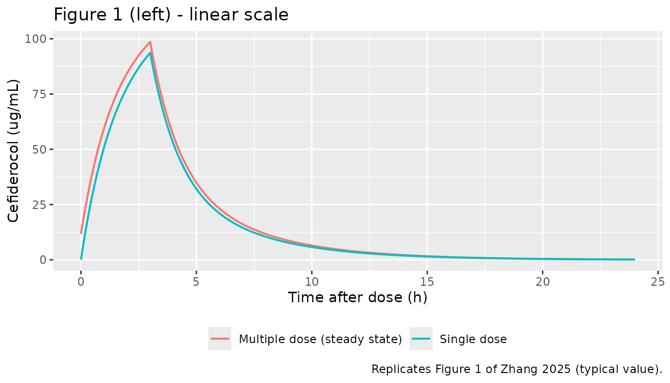
# Replicates Figure 1 (right panel) of Zhang 2025: the same profiles on a
# semi-log y axis, where the terminal slope is the hybrid rate constant beta.
p_lin +
  ggplot2::scale_y_log10() +
  ggplot2::labs(title = "Figure 1 (right) - semi-log scale")
#> Warning in ggplot2::scale_y_log10(): log-10 transformation introduced infinite
#> values.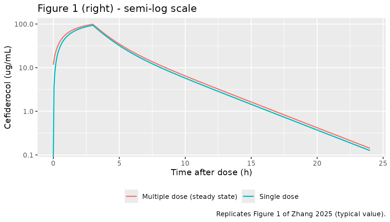
The observed profile in Figure 1 peaks at the end of the 3-h infusion and declines with a terminal half-life near 2.6 h in both arms, with the multiple-dose curve essentially superimposable on the single-dose curve apart from the non-zero pre-dose concentration. The typical-value prediction shows the same behaviour: accumulation is minimal because the dosing interval is roughly three terminal half-lives.
PKNCA validation
The source reports single-dose NCA over 0-inf and
steady-state NCA over the tau = 8 h interval following the
final dose (Table 3). Times for the multiple-dose arm are shifted so
that the final dose sits at time zero, letting both arms share a single
interval origin.
sim_nca <- sim |>
  dplyr::mutate(
    time = dplyr::if_else(treatment == "Single dose", time, time - t_last)
  ) |>
  dplyr::filter(!is.na(Cc)) |>
  dplyr::select(id, time, Cc, treatment)

# Guarantee a time = 0 row per (id, treatment). Rows already present win, which
# matters here: the steady-state arm's time-zero concentration is the trough
# carried over from the previous interval, not zero.
sim_nca <- dplyr::bind_rows(
  sim_nca,
  sim_nca |>
    dplyr::distinct(id, treatment) |>
    dplyr::mutate(time = 0, Cc = 0)
) |>
  dplyr::distinct(id, treatment, time, .keep_all = TRUE) |>
  dplyr::arrange(id, treatment, time)

# One dose row per arm at the interval origin: the day-1 dose for the
# single-dose arm, the day-5 dose for the steady-state arm.
dose_df <- data.frame(
  id = c(1L, 2L),
  time = c(0, 0),
  amt = c(dose_mg, dose_mg),
  treatment = c("Single dose", "Multiple dose (steady state)")
)

conc_obj <- PKNCA::PKNCAconc(
  sim_nca, Cc ~ time | treatment + id,
  concu = "ug/mL", timeu = "h"
)
dose_obj <- PKNCA::PKNCAdose(
  dose_df, amt ~ time | treatment + id,
  doseu = "mg"
)

nca_params <- c(
  "cmax", "tmax", "auclast", "aucinf.obs", "half.life", "cmin", "cav"
)

make_interval <- function(treatment, start, end, wanted) {
  out <- data.frame(treatment = treatment, start = start, end = end)
  for (p in nca_params) out[[p]] <- p %in% wanted
  out
}

intervals <- dplyr::bind_rows(
  make_interval(
    "Single dose", 0, Inf,
    c("cmax", "tmax", "auclast", "aucinf.obs", "half.life")
  ),
  make_interval(
    "Multiple dose (steady state)", 0, tau,
    c("cmax", "tmax", "auclast", "cmin", "cav")
  ),
  make_interval("Multiple dose (steady state)", 0, Inf, "half.life")
)

nca_res <- PKNCA::pk.nca(
  PKNCA::PKNCAdata(conc_obj, dose_obj, intervals = intervals)
)
Comparison against published NCA
Published values are the arithmetic means of the 12 participants from
Zhang 2025 Table 3. AUClast is AUC0-last for
the single-dose arm and AUC0-tau for the steady-state arm,
matching how the source labels them.
published <- tibble::tribble(
  ~treatment, ~cmax, ~tmax, ~auclast, ~aucinf.obs, ~half.life, ~cmin, ~cav,
  "Single dose", 89.44, 3.19, 384.5, 385.3, 2.53, NA, NA,
  "Multiple dose (steady state)", 92.89, 2.95, 377.8, NA, 2.67, 11.29, 47.22
)

cmp <- nlmixr2lib::ncaComparisonTable(
  simulated = nca_res,
  reference = published,
  by = "treatment",
  units = c(
    cmax = "ug/mL", cmin = "ug/mL", cav = "ug/mL", tmax = "h",
    auclast = "ug*h/mL", aucinf.obs = "ug*h/mL", half.life = "h"
  ),
  tolerance_pct = 20
)

knitr::kable(
  cmp,
  caption = paste(
    "Simulated (typical value) vs. published NCA from Zhang 2025 Table 3.",
    "* differs from reference by >20%."
  ),
  align = c("l", "l", "r", "r", "r")
)| NCA parameter | treatment | Reference | Simulated | % diff |
|---|---|---|---|---|
| Cmax (ug/mL) | Single dose | 89.4 | 93.7 | +4.8% |
| Cmax (ug/mL) | Multiple dose (steady state) | 92.9 | 98.6 | +6.1% |
| Cmin (ug/mL) | Multiple dose (steady state) | 11.3 | 11.7 | +3.5% |
| Tmax (h) | Single dose | 3.19 | 3 | -6.0% |
| Tmax (h) | Multiple dose (steady state) | 2.95 | 3 | +1.7% |
| AUC0-∞ (obs) (ug*h/mL) | Single dose | 385 | 385 | -0.1% |
| AUClast (ug*h/mL) | Single dose | 384 | 384 | -0.0% |
| AUClast (ug*h/mL) | Multiple dose (steady state) | 378 | 385 | +1.9% |
| t½ (h) | Single dose | 2.53 | 2.53 | +0.1% |
| t½ (h) | Multiple dose (steady state) | 2.67 | 2.53 | -5.2% |
| Cavg (ug/mL) | Multiple dose (steady state) | 47.2 | 48.1 | +1.9% |
pct_diff <- as.numeric(sub("%", "", sub("\\*$", "", cmp$`% diff`)))
stopifnot(!anyNA(pct_diff), nrow(cmp) == 11L)
worst <- max(abs(pct_diff))
stopifnot(worst < 10)

# Named for the prose below, so the quoted figures cannot drift from the table.
worst_rows <- cmp[order(-abs(pct_diff)), ][1:2, ]
worst_txt <- paste0(
  trimws(worst_rows[[1]]), " (", trimws(worst_rows$treatment), ", ",
  trimws(worst_rows$`% diff`), ")",
  collapse = " and "
)
cat(sprintf("Largest absolute discrepancy: %.1f%% over %d comparisons.\n",
            worst, nrow(cmp)))
#> Largest absolute discrepancy: 6.1% over 11 comparisons.
Every parameter agrees with the published mean to better than 10%,
with no row exceeding the 20% tolerance. The two largest discrepancies
are Cmax (ug/mL) (Multiple dose (steady state), +6.1%) and Tmax (h)
(Single dose, -6.0%). Both are expected consequences of comparing a
typical-value prediction against an arithmetic mean of 12 individual
fits: the model’s Tmax is exactly the end of infusion (3.00
h) whereas the observed mean Tmax reflects samples drawn at
3.0 and 3.25 h, and the observed Cmax,ss averages
individuals whose peaks are attenuated by residual assay and sampling
scatter. Notably, the typical-value Cmax after a single
dose agrees to three significant figures with the 93.7 ug/mL geometric
mean the source reports for Chinese participants in Supplementary Table
S3 - a stronger check than the arithmetic-mean comparison above, because
Table S3 is itself a model-based (NONMEM) estimate rather than a mean of
noisy individual peaks:
cmax_single <- max(sim$Cc[sim$treatment == "Single dose"], na.rm = TRUE)
stopifnot(abs(cmax_single - 93.7) / 93.7 < 0.01)
cat(sprintf(
  "Typical-value Cmax = %.2f ug/mL vs Supplementary Table S3 geometric mean 93.7 ug/mL (%.2f%% apart).\n",
  cmax_single, 100 * abs(cmax_single - 93.7) / 93.7
))
#> Typical-value Cmax = 93.71 ug/mL vs Supplementary Table S3 geometric mean 93.7 ug/mL (0.01% apart).
MIC distributions and the PK/PD target
The PK/PD analysis in the source combines this PK model with the MIC distribution of 1738 Gram-negative clinical isolates collected from five Chinese provinces in 2020 (Supplementary Table S1). Those distributions are transcribed below and used to recompute the MIC50 / MIC90 values quoted in the Results.
mic_levels <- c(0.03, 0.06, 0.12, 0.25, 0.5, 1, 2, 4, 8, 16, 32, 64)

mic_n <- c(
  "All Gram-negative" = 1738, "Enterobacterales" = 1088,
  "Pseudomonas aeruginosa" = 351, "Acinetobacter spp." = 279,
  "Stenotrophomonas maltophilia" = 20
)

# One row per organism x MIC dilution; percentages are read across the
# Supplementary Table S1 rows in the order of `mic_levels`.
mic_pct <- dplyr::bind_rows(
  data.frame(
    organism = "All Gram-negative", MIC = mic_levels,
    pct = c(16.9, 12.5, 24.6, 23.5, 11.3, 4.8, 3.5, 2.1, 0.3, 0.1, 0.1, 0.3)
  ),
  data.frame(
    organism = "Enterobacterales", MIC = mic_levels,
    pct = c(24.4, 12.7, 21.7, 15.5, 10.9, 5.7, 4.9, 3.1, 0.6, 0.0, 0.2, 0.4)
  ),
  data.frame(
    organism = "Pseudomonas aeruginosa", MIC = mic_levels,
    pct = c(2.0, 10.8, 28.5, 43.0, 11.1, 3.7, 0.9, 0.0, 0.0, 0.0, 0.0, 0.0)
  ),
  data.frame(
    organism = "Acinetobacter spp.", MIC = mic_levels,
    pct = c(3.9, 13.6, 31.2, 31.5, 13.3, 2.9, 1.8, 1.1, 0.0, 0.4, 0.0, 0.4)
  ),
  data.frame(
    organism = "Stenotrophomonas maltophilia", MIC = mic_levels,
    pct = c(50.0, 15.0, 25.0, 5.0, 5.0, 0.0, 0.0, 0.0, 0.0, 0.0, 0.0, 0.0)
  )
)

mic_quantile <- function(mic, pct, target) {
  idx <- which(cumsum(pct) >= target)[1]
  if (is.na(idx)) NA_real_ else mic[idx]
}

mic_summary <- mic_pct |>
  dplyr::arrange(organism, MIC) |>
  dplyr::group_by(organism) |>
  dplyr::summarise(
    MIC50 = mic_quantile(MIC, pct, 50),
    MIC90 = mic_quantile(MIC, pct, 90),
    .groups = "drop"
  ) |>
  dplyr::mutate(n = unname(mic_n[organism])) |>
  dplyr::select(organism, n, MIC50, MIC90)

mic_summary |>
  dplyr::rename(
    "Organism" = organism,
    "N isolates" = n,
    "MIC50 (ug/mL)" = MIC50,
    "MIC90 (ug/mL)" = MIC90
  ) |>
  knitr::kable(
    caption = paste(
      "MIC50 / MIC90 recomputed from the Supplementary Table S1 distributions.",
      "The lowest tested dilution is reported by the source as <=0.03 ug/mL."
    )
)| Organism | N isolates | MIC50 (ug/mL) | MIC90 (ug/mL) |
|---|---|---|---|
| Acinetobacter spp. | 279 | 0.25 | 0.50 |
| All Gram-negative | 1738 | 0.12 | 1.00 |
| Enterobacterales | 1088 | 0.12 | 1.00 |
| Pseudomonas aeruginosa | 351 | 0.25 | 0.50 |
| Stenotrophomonas maltophilia | 20 | 0.03 | 0.12 |
# The source states these MIC50 / MIC90 pairs in Results, "MIC Distribution of
# Cefiderocol Against Gram-Negative Clinical Isolates in China".
mic_reference <- tibble::tribble(
  ~organism, ~MIC50, ~MIC90,
  "Enterobacterales", 0.12, 1,
  "Pseudomonas aeruginosa", 0.25, 0.5,
  "Acinetobacter spp.", 0.25, 0.5,
  "Stenotrophomonas maltophilia", 0.03, 0.12
)

mic_check <- dplyr::inner_join(
  mic_reference, mic_summary,
  by = "organism", suffix = c("_published", "_recomputed")
)
stopifnot(
  nrow(mic_check) == nrow(mic_reference),
  isTRUE(all.equal(mic_check$MIC50_published, mic_check$MIC50_recomputed)),
  isTRUE(all.equal(mic_check$MIC90_published, mic_check$MIC90_recomputed))
)
cat(sprintf(
  "All %d published MIC50/MIC90 pairs reproduced from Table S1.\n",
  nrow(mic_check)
))
#> All 4 published MIC50/MIC90 pairs reproduced from Table S1.
All four published MIC50 / MIC90 pairs are reproduced exactly from the Supplementary Table S1 percentages, confirming the transcription.
Time above MIC for the typical participant
The source’s PD index is %fT>MIC - the fraction of
the dosing interval during which the unbound
concentration exceeds the MIC - with a 75.0% target for all
Gram-negative pathogens and organism-specific targets of 73.3%
(Enterobacterales), 72.2% (P. aeruginosa), 88.1%
(A. baumannii) and 53.9% (S. maltophilia).
The unbound fraction of cefiderocol is not reported anywhere in the
paper or its supplement, so the free-drug index cannot be computed from
the published sources. The table below therefore reports
%T>MIC on total plasma concentration
for the typical participant at steady state. It is an upper bound on
%fT>MIC, not a reproduction of the published target
attainment; see Assumptions and deviations.
ss_profile <- sim |>
  dplyr::filter(treatment == "Multiple dose (steady state)", !is.na(Cc)) |>
  dplyr::mutate(tad = time - t_last) |>
  dplyr::filter(tad >= 0, tad <= tau) |>
  dplyr::arrange(tad)

pct_t_above <- function(mic) {
  above <- ss_profile$Cc > mic
  # Trapezoidal fraction of the interval spent above the MIC.
  dt <- diff(ss_profile$tad)
  mid <- (head(above, -1) + tail(above, -1)) / 2
  100 * sum(dt * mid) / tau
}

t_above <- tibble::tibble(
  MIC = c(0.25, 0.5, 1, 2, 4, 8, 16),
  `%T>MIC (total drug)` = vapply(MIC, pct_t_above, numeric(1))
)

t_above |>
  dplyr::rename("MIC (ug/mL)" = MIC) |>
  knitr::kable(
    digits = 1,
    caption = paste(
      "Percentage of the 8-h steady-state interval with total cefiderocol",
      "above the MIC, typical participant, 2 g q8h over 3 h."
    )
)| MIC (ug/mL) | %T>MIC (total drug) |
|---|---|
| 0.2 | 100.0 |
| 0.5 | 100.0 |
| 1.0 | 100.0 |
| 2.0 | 100.0 |
| 4.0 | 100.0 |
| 8.0 | 100.0 |
| 16.0 | 86.9 |
# Trough at steady state is 11.68 ug/mL, so total-drug T>MIC must be 100% at
# every MIC below it and strictly decreasing above it.
stopifnot(
  all(t_above$`%T>MIC (total drug)`[t_above$MIC <= 8] == 100),
  t_above$`%T>MIC (total drug)`[t_above$MIC == 16] < 100
)
Because the typical steady-state trough is 11.7 ug/mL, total-drug
T>MIC is 100% for every MIC up to 8 ug/mL. This is
precisely why the published analysis needs between-subject variability:
for a single typical participant the attainment curve is a step
function, and the shape of the published PTA curve is carried entirely
by the parameter distribution that the source did not report.
Assumptions and deviations
The model is packaged in the source’s macro-constant parameterisation. Supplementary Table S2 reports
V1,K21,AlphaandBeta; those four values are transcribed verbatim, andkel,k12,CL,QandVpare derived insidemodel()from the standard identitiesalpha + beta = kel + k12 + k21andalpha * beta = kel * k21. The derived typical values (CL5.197 L/h,Q1.437 L/h,Vp3.422 L) are not printed in the source; they reproduce the published noncompartmentalCL(5.32 L/h),Vz(19.4 L) andt1/2,z(2.53 h) to within 3%.-
Between-subject variability is encoded as
fixed(0)and cannot be simulated. Supplementary Table S2 reports an arithmetic SD next to each parameter (V1CV 15.3%,K21CV 26.0%,AlphaCV 22.1%,BetaCV 14.4%), and the Monte Carlo simulation behind the published PTA and CFR results sampled 5000 virtual participants from those parameters while, in the authors’ words, “considering correlation among PK parameters”. The correlation matrix is reported nowhere in the paper or its supplement, and the marginal SDs cannot be used without it: a valid two-compartment parameter set requiresalpha > k21 > beta, and drawing the three rate constants independently from the reported marginals violates that ordering in roughly 9% of draws (yielding a negativek12; recomputed below). Encoding the marginals as independent etas would therefore both misrepresent the authors’ simulation and generate structurally invalid participants. The etas are declared and fixed at zero so that the reported spread is recorded without inventing a variance-covariance structure;fixed(0)here means “joint distribution unreported”, not “the authors observed zero variability”.The ordering-violation rate quoted above is recomputed here rather than asserted, under both readings of the reported SDs:
set.seed(20250313)
n_draw <- 2e5
draw_violation <- function(to_sdlog) {
  al <- 0.845 * exp(rnorm(n_draw, 0, to_sdlog(0.187 / 0.845)))
  k21 <- 0.420 * exp(rnorm(n_draw, 0, to_sdlog(0.109 / 0.420)))
  be <- 0.271 * exp(rnorm(n_draw, 0, to_sdlog(0.039 / 0.271)))
  100 * mean(al + be - k21 - al * be / k21 <= 0) # k12 <= 0
}
viol_lognormal <- draw_violation(function(cv) sqrt(log(1 + cv^2)))

set.seed(20250313)
al <- rnorm(n_draw, 0.845, 0.187)
k21 <- rnorm(n_draw, 0.420, 0.109)
be <- rnorm(n_draw, 0.271, 0.039)
viol_normal <- 100 * mean(al + be - k21 - al * be / k21 <= 0)

stopifnot(viol_lognormal > 5, viol_lognormal < 15, viol_normal > 5)
cat(sprintf(
  "Independent draws give a structurally invalid k12 in %.1f%% (lognormal) / %.1f%% (normal) of subjects.\n",
  viol_lognormal, viol_normal
))
#> Independent draws give a structurally invalid k12 in 8.6% (lognormal) / 12.3% (normal) of subjects.
The published PTA and CFR results are not reproduced here, by design. They depend on the unreported parameter correlation above and on an unbound fraction that the source never states. Reproducing Figure 3, Figure S1 or Table 4 would require supplying both from outside the paper. The MIC distributions in Supplementary Table S1 and the published MIC50 / MIC90 values are reproduced, and the
%T>MICtable reports total drug with that limitation stated explicitly.No residual-error model is available. The source summarises individual WinNonlin curve fits as mean (SD) rather than fitting a population model with a residual-error component, so
propSdisfixed(0).No covariate effects. All 12 participants were healthy Chinese adults with normal renal function receiving an identical regimen, and the source reports no covariate screen. Cefiderocol clearance is known to depend strongly on renal function, but nothing in this paper supports such a term; the model should not be extrapolated to renal impairment.
Simulated arms are typical-value predictions, not virtual populations. With all etas at zero, one deterministic subject per arm carries the whole prediction, so the comparison in the NCA table is a typical value against the published arithmetic mean of 12 participants rather than a distributional comparison.
Steady state is assumed reached by the 21st dose. The source dosed q8h from day 2 to the morning of day 5 and confirmed steady state by ANOVA on trough concentrations. With a terminal half-life of 2.55 h, the simulation reaches steady state well before the final dose at
t = 160 h.All parameter values come from the paper and its supplement. No value in this model was digitised from a figure, obtained by author correspondence, or carried from an upstream publication.