TDI01 (Ji 2025) • nlmixr2lib

Model and source

Citation: Ji X, Cui Y. Model-informed drug development of novel ROCK2 inhibitor TDI01: population pharmacokinetic study and simulation. Front Pharmacol. 2025;16:1477607. doi:10.3389/fphar.2025.1477607.
Description: Population PK model for orally administered TDI01, a novel selective ROCK2 inhibitor developed for acute lung injury / acute respiratory distress syndrome (ALI/ARDS), in healthy Chinese adults (Ji 2025, final Pop-PK model). Disposition is one-compartment with first-order absorption plus a gallbladder compartment that reproduces the double-peak hepato-enteral (enterohepatic) circulation seen after single dosing: drug leaves the central compartment continuously into the gallbladder at the fixed rate k2G, and the gallbladder discharges back into the absorption compartment at the fixed rate kG1 only while the authors’ FLAG time switch is open, which they set to the 8-10 h post-dose window. All disposition parameters are apparent (per unit bioavailability, /F). No covariate model was developed because the phase 1 population was demographically homogeneous. Note that the source describes the final model as a one-compartment model ‘with dosage effect’, reporting that relative bioavailability was higher at 200-400 mg than at 800-1,200 mg, but it tabulates no dose-effect parameter and writes no dose term into its published equations; the packaged model therefore carries F = 1 at every dose. See the vignette ‘Assumptions and deviations’ section.
Article: https://doi.org/10.3389/fphar.2025.1477607

TDI01 is a selective Rho-associated coiled-coil-containing protein kinase 2 (ROCK2) inhibitor developed for acute lung injury / acute respiratory distress syndrome. Ji and Cui fitted a population PK model to a phase 1 single- and multiple-ascending-dose study, then used it to simulate two candidate 7-day regimens.

The defining feature of the data is a double-peak concentration-time profile after a single oral dose, which the authors attributed to hepato-enteral (enterohepatic) circulation. Their structural model therefore carries a gallbladder compartment that fills continuously from the central compartment and discharges back into the absorption compartment during a 2 h window, gated by a time switch the paper calls FLAG.

There is no supplementary material and no published erratum for this article (checked 2026-08-14); the model specification is contained entirely in the paper’s Table 1 and Equations 1-5.

Population

The model was fitted to 776 quantifiable plasma concentrations from 39 healthy Chinese volunteers in a single phase 1 study, sponsored by Beijing Tide Pharmaceutical Co., Ltd. and conducted at the Institute of Clinical Pharmacology, Peking University First Hospital. Single-dose arms received 400, 800, or 1,200 mg orally; multiple-dose arms received 200 mg QD or 400 mg QD for 7 days. Single-dose arms were sampled pre-dose and at 1, 2, 3, 3.5, 4, 5, 6, 8, 10, 12, 24, 36, 48, and 72 h; multiple-dose arms were sampled out to 216 h with a dense schedule bracketing the day-7 dose.

Ten of 786 observations (1.3%) were below the limit of quantification; because that is under the paper’s 10% threshold, they were excluded rather than handled by a likelihood-based method. Observations with |CWRES| > 5 were treated as outliers during model building and re-introduced for a sensitivity analysis.

The paper publishes no baseline demographic table. Age, body weight, sex, and BMI distributions are not reported; the only characterisation given is that the cohort had a “homogeneous demographic profile” (Discussion, Limitations). Consequently no covariate model was developed, and the population metadata for this model deliberately omits those fields rather than guessing them. The virtual cohort below therefore varies only the model’s own random effects.

pop <- rxode2::rxode(readModelDb("Ji_2025_TDI01"))$population
#> ℹ parameter labels from comments will be replaced by 'label()'
str(pop, max.level = 1)
#> List of 9
#>  $ species        : chr "human"
#>  $ n_subjects     : int 39
#>  $ n_observations : int 776
#>  $ n_studies      : int 1
#>  $ disease_state  : chr "Healthy volunteers."
#>  $ dose_range     : chr "Oral TDI01. Single-dose regimens: 400 mg, 800 mg, and 1,200 mg. Multiple-dose regimens: 200 mg QD for 7 days an"| __truncated__
#>  $ regions        : chr "China (Institute of Clinical Pharmacology, Peking University First Hospital, Beijing; sponsor Beijing Tide Phar"| __truncated__
#>  $ sampling_window: chr "Single-dose groups: 0 (pre-dose), 1, 2, 3, 3.5, 4, 5, 6, 8, 10, 12, 24, 36, 48, 72 h post-dose. Multiple-dose g"| __truncated__
#>  $ notes          : chr "The source reports NO baseline demographic table: age, body weight, sex, and body-mass-index distributions are "| __truncated__

Source trace

The per-parameter origin is recorded as an in-file comment next to each ini() entry in inst/modeldb/specificDrugs/Ji_2025_TDI01.R. The table below collects them in one place for review.

Equation / parameter	Value	Source location
`lcl` (CL/F)	95 L/h	Table 1, “CL/F (L/h)”, Final model (RSE 10%)
`lvc` (Vc/F)	1,400 L	Table 1, “Vc/F (L)”, Final model (RSE 8%)
`lka` (ka/F)	0.345 1/h	Table 1, “ka/F (1/h)”, Final model (RSE 10%)
`lkbm` (k2G/F)	0.023 1/h, FIXED	Table 1, “k2G/F (1/h)” = 0.023 (FIX)
`lkehc` (kG1/F)	2 1/h, FIXED	Table 1, “kG1/F (1/h)” = 2 (FIX)
`ltgb` (FLAG onset)	8 h post-dose, FIXED	Results: “the starting and ending time of hepato-enteral circulation was set as 8-10 h”
`ldgb` (FLAG duration)	2 h, FIXED	Results, same sentence (10 h - 8 h)
`etalcl`	0.198051 = log(1 + 0.468^2)	Table 1, “IIV_CL/F” = 46.8% CV; Methods Equation 1 (exponential IIV)
`etalvc`	0.098654 = log(1 + 0.322^2)	Table 1, “IIV_V/F” = 32.2% CV; Methods Equation 1
`etalka`	0.201903 = log(1 + 0.473^2)	Table 1, “IIV_k12” = 47.3% CV; Methods Equation 1 (see note below)
`propSd`	0.342	Table 1, “Prop.error (%)” = 34.2% (RSE 3%); Methods Equation 2
`addSd`	1.77 ng/mL	Table 1, “Add.error” = 1.77 (RSE 47%); Methods Equation 2
`kel <- cl / vc`	n/a	Line preceding Equation 3: “K20 = CL/Vc”
`d/dt(depot)`	n/a	Equation 3: `DADT(1) = FLAGKG1A(2) - Ka*A`
`d/dt(central)`	n/a	Equation 4: `DADT(2) = KaA - K2GA(1) - K20*A(1)`
`d/dt(gallbladder)`	n/a	Equation 5: `DADT(3) = K2GA(1) - FLAGKG1*A(2)`
`Cc <- central / vc * 1000`	n/a	Unit conversion mg/L -> ng/mL; concentration scale set by Table 3 (ng/mL) and Add.error = 1.77

Two transcription decisions in that table deserve their reasoning spelled out.

Compartment indexing. Equations 3-5 use DADT(1) / DADT(2) / DADT(3) on the left-hand side but A / A(1) / A(2) on the right, and the legend states that “A, A (1) and A (2) represent absorption, central and gallbladder compartments, respectively”. Reading the right-hand sides under that legend, the three equations are internally consistent and map unambiguously onto depot / central / gallbladder: every gallbladder loss term is exactly the matching depot gain term, and the central loss to bile is exactly the gallbladder gain. Mass balance therefore closes, so the index offset between the DADT(n) and A(n) notations is a typographic artifact rather than a genuine ambiguity.

IIV_k12. Table 1’s third variance component is labelled IIV_k12, a name that appears nowhere in Equations 3-5. It is the IIV on ka: k12 is the NONMEM micro-constant for transfer from compartment 1 (depot) to compartment 2 (central), which is ka; and ka is the only estimated structural parameter left once IIV_CL/F and IIV_V/F are assigned, because k2G and kG1 are both FIX and so cannot carry a variance.

Virtual cohort

Original observed data are not publicly available. The figures below use virtual cohorts of 200 subjects per arm (the per-arm cap for this repository), varying only the model’s own between-subject random effects on CL/F, Vc/F, and ka – the paper reports no covariates and no demographic distributions to sample from.

set.seed(20250304)

n_arm <- 200L

# One arm as a self-contained event table. `id_offset` keeps IDs disjoint
# across arms; duplicate IDs across arms would silently collapse into single
# subjects that receive the summed dose.
make_arm <- function(amt, ii, addl, label, obs_times, id_offset = 0L) {
  ev <- rxode2::et(amt = amt, ii = ii, addl = addl, cmt = "depot") |>
    rxode2::et(obs_times, cmt = "central") |>
    rxode2::et(id = id_offset + seq_len(n_arm))
  as.data.frame(ev) |>
    dplyr::mutate(regimen = label)
}

# --- single ascending doses (paper Figure 4) -------------------------------
sd_times <- sort(unique(c(seq(0, 14, by = 0.25), seq(14, 72, by = 0.5))))

events_sd <- dplyr::bind_rows(
  make_arm(400,  ii = 0, addl = 0, "400 mg single",   sd_times, id_offset = 0L),
  make_arm(800,  ii = 0, addl = 0, "800 mg single",   sd_times, id_offset = 1000L),
  make_arm(1200, ii = 0, addl = 0, "1,200 mg single", sd_times, id_offset = 2000L)
)
stopifnot(!anyDuplicated(events_sd[, c("id", "time", "evid")]))

# --- multiple ascending doses + the two simulated regimens (Figures 5, 6) ---
# Dense sampling brackets the day-7 dose (144 h) so the steady-state interval
# is well resolved for NCA.
md_times <- sort(unique(c(seq(0, 24, by = 0.5), seq(24, 144, by = 2),
                          seq(144, 168, by = 0.25), seq(168, 216, by = 1))))

events_md <- dplyr::bind_rows(
  make_arm(200, ii = 24, addl =  6, "200 mg QD, 7 d",  md_times, id_offset = 0L),
  make_arm(400, ii = 24, addl =  6, "400 mg QD, 7 d",  md_times, id_offset = 1000L),
  make_arm(200, ii = 12, addl = 13, "200 mg BID, 7 d", md_times, id_offset = 2000L)
)
stopifnot(!anyDuplicated(events_md[, c("id", "time", "evid")]))

c(single_dose_rows = nrow(events_sd), multiple_dose_rows = nrow(events_md))
#>   single_dose_rows multiple_dose_rows 
#>             104400             152400

Simulation

mod <- readModelDb("Ji_2025_TDI01")

sim_sd <- rxode2::rxSolve(mod, events = events_sd, keep = "regimen") |>
  as.data.frame()
#> ℹ parameter labels from comments will be replaced by 'label()'
sim_md <- rxode2::rxSolve(mod, events = events_md, keep = "regimen") |>
  as.data.frame()

# Typical-value (deterministic) profiles: supply zero eta columns and switch
# off the sampler with omega = NA. This is preferred over zeroRe(), which
# mutates shared model state.
etas0 <- data.frame(id = 1L, etalcl = 0, etalvc = 0, etalka = 0)

solve_typical <- function(amt, ii, addl, obs_times, pars = NULL) {
  ev <- rxode2::et(amt = amt, ii = ii, addl = addl, cmt = "depot") |>
    rxode2::et(obs_times, cmt = "central")
  rxode2::rxSolve(mod, ev, etas0, omega = NA, params = pars,
                  atol = 1e-10, rtol = 1e-10) |>
    as.data.frame()
}

Replicate published figures

Figure 1 – dose-normalised profiles

Figure 1 of Ji 2025 overlays dose-normalised concentration-time profiles from every arm. In the observed data the low-dose arms sit above the high-dose arms, which is the observation the authors cite as evidence of a “dosage effect” on bioavailability. The packaged model is strictly linear in dose (f(depot) is unity at every dose and every term is first-order), so its dose-normalised profiles superimpose exactly. That superposition is the cleanest available demonstration that the dose effect described in the text was never quantified into a parameter – see Assumptions and deviations.

# Replicates Figure 1 of Ji 2025: dose-normalised concentration-time profiles.
dose_of <- c("400 mg single" = 400, "800 mg single" = 800,
             "1,200 mg single" = 1200)

sim_sd |>
  dplyr::filter(!is.na(Cc)) |>
  dplyr::mutate(Cc_norm = Cc / dose_of[as.character(regimen)]) |>
  dplyr::group_by(time, regimen) |>
  dplyr::summarise(Q50 = median(Cc_norm), .groups = "drop") |>
  ggplot(aes(time, Q50, colour = regimen)) +
  geom_line(linewidth = 0.9) +
  labs(x = "Time (h)", y = "Dose-normalised Cc (ng/mL per mg)",
       colour = "Regimen",
       title = "Figure 1 -- dose-normalised single-dose profiles",
       caption = paste("Replicates Figure 1 of Ji 2025. The three curves",
                       "superimpose because the packaged model is linear in",
                       "dose; the paper's observed curves do not.")) +
  theme(legend.position = "bottom")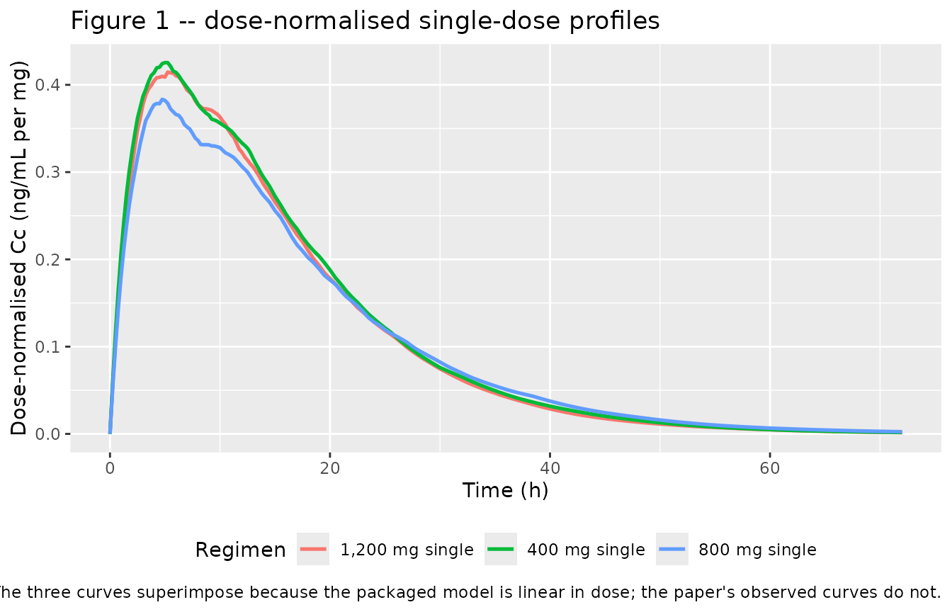

Figures 4 and 5 – visual predictive checks

# Replicates Figure 4 of Ji 2025: VPC of single ascending doses.
vpc <- function(d) {
  d |>
    dplyr::filter(!is.na(Cc)) |>
    dplyr::group_by(time, regimen) |>
    dplyr::summarise(Q025 = quantile(Cc, 0.025), Q50 = median(Cc),
                     Q975 = quantile(Cc, 0.975), .groups = "drop")
}

vpc(sim_sd) |>
  ggplot(aes(time, Q50)) +
  geom_ribbon(aes(ymin = Q025, ymax = Q975), alpha = 0.25, fill = "steelblue") +
  geom_line(colour = "steelblue", linewidth = 0.8) +
  facet_wrap(~regimen) +
  labs(x = "Time (h)", y = "Cc (ng/mL)",
       title = "Figure 4 -- VPC, single ascending doses",
       caption = paste("Replicates Figure 4 of Ji 2025 (arithmetic scale).",
                       "Median and 95% prediction interval, 200 subjects/arm."))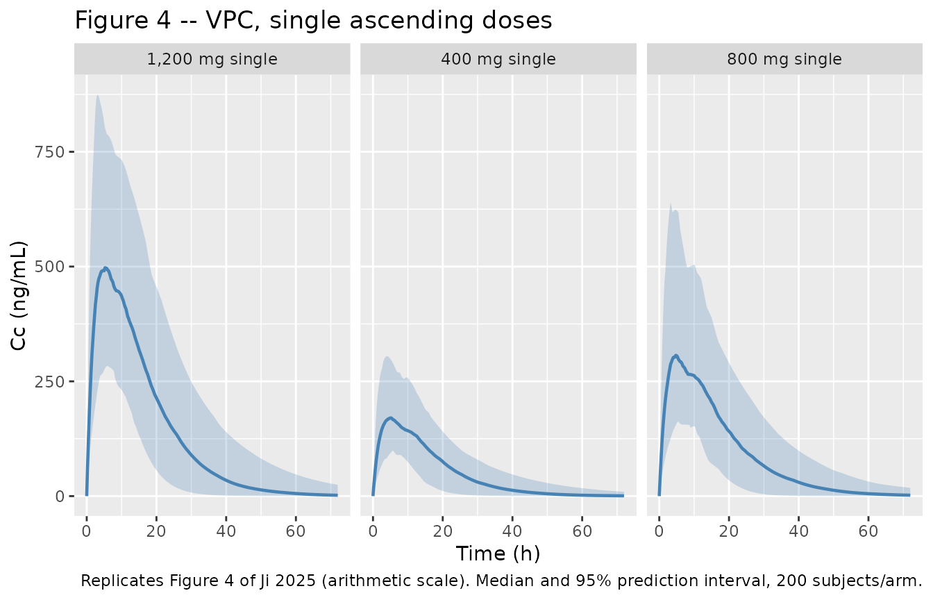

# Figure 4B of Ji 2025: the same VPC on a logarithmic concentration scale.
vpc(sim_sd) |>
  dplyr::filter(time > 0) |>
  ggplot(aes(time, Q50)) +
  geom_ribbon(aes(ymin = Q025, ymax = Q975), alpha = 0.25, fill = "steelblue") +
  geom_line(colour = "steelblue", linewidth = 0.8) +
  facet_wrap(~regimen) +
  scale_y_log10() +
  labs(x = "Time (h)", y = "Cc (ng/mL, log scale)",
       title = "Figure 4B -- VPC, single ascending doses (log scale)",
       caption = "Replicates Figure 4B of Ji 2025.")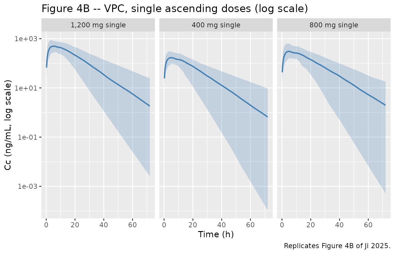

# Replicates Figure 5 of Ji 2025: VPC of multiple ascending doses (the two
# clinical multiple-dose arms, 200 mg QD and 400 mg QD for 7 days).
vpc(sim_md) |>
  dplyr::filter(regimen %in% c("200 mg QD, 7 d", "400 mg QD, 7 d")) |>
  ggplot(aes(time, Q50)) +
  geom_ribbon(aes(ymin = Q025, ymax = Q975), alpha = 0.25, fill = "darkorange") +
  geom_line(colour = "darkorange3", linewidth = 0.8) +
  facet_wrap(~regimen, ncol = 1) +
  labs(x = "Time (h)", y = "Cc (ng/mL)",
       title = "Figure 5 -- VPC, multiple ascending doses",
       caption = paste("Replicates Figure 5 of Ji 2025. Doses at 0-144 h;",
                       "sampling continues to 216 h."))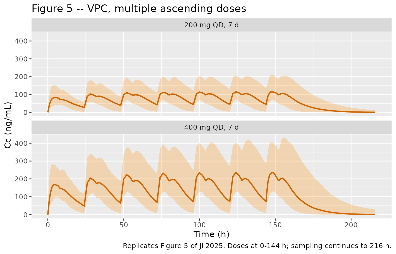

Figure 6 – the two simulated candidate regimens

# Replicates Figure 6 of Ji 2025: simulated profiles for the two designed
# regimens over the 7-day treatment course.
vpc(sim_md) |>
  dplyr::filter(regimen %in% c("400 mg QD, 7 d", "200 mg BID, 7 d")) |>
  ggplot(aes(time, Q50, colour = regimen, fill = regimen)) +
  geom_ribbon(aes(ymin = Q025, ymax = Q975), alpha = 0.2, colour = NA) +
  geom_line(linewidth = 0.8) +
  geom_hline(yintercept = 1391, linetype = "dashed") +
  annotate("text", x = 20, y = 1391, vjust = -0.5, size = 3,
           label = "observed Cmax at 1,200 mg single dose = 1,391 ng/mL") +
  labs(x = "Time (h)", y = "Cc (ng/mL)", colour = "Regimen", fill = "Regimen",
       title = "Figure 6 -- simulated candidate regimens",
       caption = paste("Replicates Figure 6 of Ji 2025. The dashed line is the",
                       "safety benchmark the paper compares against.")) +
  theme(legend.position = "bottom")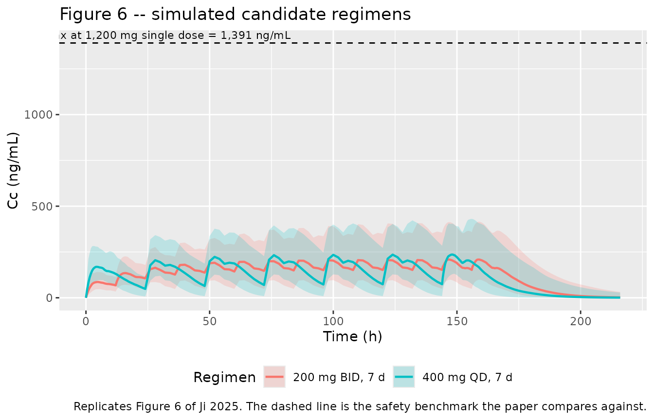

The paper’s safety argument is that concentrations under both 7-day regimens stay below the 1,391 ng/mL Cmax observed at the highest single dose. The packaged model reproduces that conclusion, and with a wide margin.

Structural checks

Three quantitative gates exercise parts of the model that a visual profile check cannot. The first two are exact identities; the third confirms the enterohepatic loop is actually live rather than silently inert.

Closed-form steady-state mass balance

Because every molecule that enters the gallbladder is eventually released back into the depot and cleared only through CL/F, the steady-state exposure over a 24 h period must equal the daily dose divided by apparent clearance, independently of the recirculation parameters:

$\mathrm{AUC}_{0-24,ss} = \frac{D_{\text{daily}}}{\mathrm{CL}/F}$

This is a strong gate: it fails if the recirculation is leaking mass, if the FLAG window never reopens, or if the mg/L-to-ng/mL scaling is wrong.

auc_trap <- function(d) sum(diff(d$time) * (head(d$Cc, -1) + tail(d$Cc, -1)) / 2)

ss_window <- seq(144, 168, by = 0.05)

mb <- dplyr::bind_rows(
  lapply(
    list(list("400 mg QD, 7 d", 400, 24, 6), list("200 mg BID, 7 d", 200, 12, 13)),
    function(r) {
      d <- solve_typical(r[[2]], r[[3]], r[[4]], ss_window) |>
        dplyr::filter(time >= 144, time <= 168)
      data.frame(regimen = r[[1]],
                 simulated = auc_trap(d),
                 closed_form = (24 / r[[3]]) * r[[2]] / 95 * 1000)
    }
  )
) |>
  dplyr::mutate(pct_diff = 100 * (simulated - closed_form) / closed_form)

mb |>
  dplyr::rename("Regimen" = regimen,
                "Simulated AUC0-24,ss (ng*h/mL)" = simulated,
                "Dose_daily / (CL/F) (ng*h/mL)"  = closed_form,
                "% diff" = pct_diff) |>
  knitr::kable(digits = c(0, 1, 1, 3),
               caption = "Steady-state AUC against the closed-form identity.")

Steady-state AUC against the closed-form identity.
Regimen	Simulated AUC0-24,ss (ng*h/mL)	Dose_daily / (CL/F) (ng*h/mL)	% diff
400 mg QD, 7 d	4207.8	4210.5	-0.065
200 mg BID, 7 d	4209.7	4210.5	-0.020


stopifnot(all(abs(mb$pct_diff) < 0.5))

Both regimens agree with the closed form to better than 0.5%, and they agree with each other – which is expected, because 400 mg QD and 200 mg BID deliver the same 400 mg daily dose. Hold on to that fact; it matters when the paper’s own Table 3 is compared below.

Analytic Tmax and terminal half-life

Before the FLAG window opens at 8 h the gallbladder is a pure sink, so the single-dose system is exactly a one-compartment oral model with total central exit rate $k = k_{el} + k_{2G}$ . Tmax and the terminal slope therefore have closed forms, and Tmax (5.25 h) falls before the window opens, so the recirculation cannot perturb it.

cl <- 95; vc <- 1400; ka <- 0.345; k2g <- 0.023
k  <- cl / vc + k2g

tmax_analytic <- log(ka / k) / (ka - k)
thalf_analytic <- log(2) / k

d1200 <- solve_typical(1200, 0, 0, seq(0, 72, by = 0.01))
tmax_sim <- d1200$time[which.max(d1200$Cc)]

tail_fit <- d1200 |> dplyr::filter(time >= 40, time <= 70)
thalf_sim <- log(2) / -coef(lm(log(Cc) ~ time, data = tail_fit))[["time"]]

data.frame(
  quantity  = c("Tmax (h)", "Terminal half-life (h)"),
  analytic  = c(tmax_analytic, thalf_analytic),
  simulated = c(tmax_sim, thalf_sim)
) |>
  dplyr::mutate("% diff" = 100 * (simulated - analytic) / analytic) |>
  dplyr::rename("Quantity" = quantity, "Analytic" = analytic,
                "Simulated" = simulated) |>
  knitr::kable(digits = 3,
               caption = "Single-dose Tmax and terminal half-life vs. closed form.")

Single-dose Tmax and terminal half-life vs. closed form.
Quantity	Analytic	Simulated	% diff
Tmax (h)	5.250	5.250	0.000
Terminal half-life (h)	7.629	7.629	0.002


stopifnot(abs(tmax_sim - tmax_analytic) < 0.05,
          abs(thalf_sim - thalf_analytic) / thalf_analytic < 0.01)

The enterohepatic loop is live

A named intermediate that gates an ODE term can silently evaluate to zero, in which case the whole recirculation would vanish without any error. This gate ablates biliary uptake (k2G set near zero) and confirms that the gallbladder state, and the concentration trajectory, both respond.

d_ehc  <- solve_typical(1200, 0, 0, seq(0, 48, by = 0.05))
d_none <- solve_typical(1200, 0, 0, seq(0, 48, by = 0.05),
                        pars = c(lkbm = log(1e-12)))

gb_peak  <- max(d_ehc$gallbladder[d_ehc$time <= 8])
gb_after <- d_ehc$gallbladder[which.min(abs(d_ehc$time - 10))]

data.frame(
  quantity = c("Gallbladder amount at 8 h, FLAG onset (mg)",
               "Gallbladder amount at 10 h, FLAG close (mg)",
               "Fraction of the gallbladder emptied in the window",
               "Gallbladder peak with k2G ablated (mg)"),
  value = c(gb_peak, gb_after, 1 - gb_after / gb_peak,
            max(d_none$gallbladder))
) |>
  dplyr::rename("Quantity" = quantity, "Value" = value) |>
  knitr::kable(digits = 4, caption = "Ablation check on the enterohepatic loop.")

Ablation check on the enterohepatic loop.
Quantity	Value
Gallbladder amount at 8 h, FLAG onset (mg)	111.2948
Gallbladder amount at 10 h, FLAG close (mg)	9.4683
Fraction of the gallbladder emptied in the window	0.9149
Gallbladder peak with k2G ablated (mg)	0.0000


# The loop must move a material amount of drug, and must vanish when ablated.
stopifnot(gb_peak > 100,                       # >100 mg of the 1,200 mg dose
          1 - gb_after / gb_peak > 0.9,        # window empties >90% of it
          max(d_none$gallbladder) < 1e-3)      # ablation kills the loop

The recirculation moves 111 mg of the 1,200 mg dose and discharges over 90% of it during the 2 h window, and ablating k2G removes the loop entirely. The mechanism is therefore live.

What the recirculation does not do

With the published parameter values the recirculation does not produce a visible second peak. The recycled bolus re-enters the depot and must then be absorbed at ka = 0.345 1/h (2.0 h half-life) into a central compartment that is still holding roughly 700 mg and declining with a 7.6 h half-life, so the returning mass changes the curvature without ever reversing the slope.

sig <- d_ehc |>
  dplyr::select(time, Cc_ehc = Cc) |>
  dplyr::inner_join(d_none |> dplyr::select(time, Cc_none = Cc), by = "time") |>
  dplyr::mutate(ratio = Cc_ehc / Cc_none)

n_peaks <- function(x) sum(diff(sign(diff(x))) == -2)
at <- function(tt) sig$ratio[which.min(abs(sig$time - tt))]

# The recirculation's signature is a LOCAL minimum in the ratio at the FLAG
# onset followed by a rise as recycled drug is reabsorbed. It is not the
# global minimum over the whole profile: after a single dose the window never
# reopens, so biliary uptake continuing past 10 h is permanently stranded and
# the ratio resumes falling (quantified in the next chunk).
local_win <- sig |> dplyr::filter(time >= 4, time <= 14)
t_local_min <- local_win$time[which.min(local_win$ratio)]

cat(sprintf("local maxima in Cc: with EHC = %d, with k2G ablated = %d\n",
            n_peaks(d_ehc$Cc[d_ehc$time > 0]),
            n_peaks(d_none$Cc[d_none$time > 0])))
#> local maxima in Cc: with EHC = 1, with k2G ablated = 1
cat(sprintf("ratio on [4, 14] h is minimised at t = %.2f h (FLAG onset is 8 h)\n",
            t_local_min))
#> ratio on [4, 14] h is minimised at t = 8.20 h (FLAG onset is 8 h)
cat(sprintf("ratio: %.4f at 8.5 h -> %.4f at 12 h (rise = recycled drug reabsorbed)\n",
            at(8.5), at(12)))
#> ratio: 0.8854 at 8.5 h -> 0.9364 at 12 h (rise = recycled drug reabsorbed)

stopifnot(t_local_min >= 8, t_local_min <= 9,   # local min sits at the onset
          at(12) > at(8.5),                     # then rises as drug reabsorbs
          n_peaks(d_ehc$Cc[d_ehc$time > 0]) == 1L)  # but never a second peak

ggplot(sig |> dplyr::filter(time > 0), aes(time, ratio)) +
  geom_vline(xintercept = c(8, 10), linetype = "dotted") +
  geom_line(linewidth = 0.8, colour = "purple4") +
  labs(x = "Time (h)", y = "Cc with EHC / Cc with k2G ablated",
       title = "Signature of the recirculation on a single 1,200 mg dose",
       caption = paste("Dotted lines bracket the 8-10 h FLAG window. The ratio",
                       "dips to a local minimum at the window onset and rises",
                       "as recycled drug is reabsorbed, then falls again as",
                       "post-window biliary uptake is stranded."))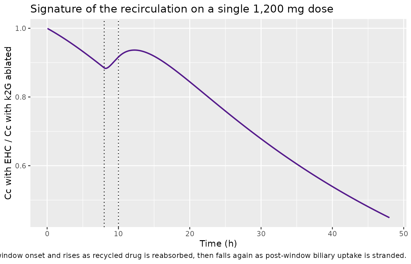

After a single dose the FLAG window opens exactly once, so any drug taken up into bile after 10 h stays there permanently. That is a real property of the published model rather than an artifact of this implementation, and it means single-dose AUC falls short of D/(CL/F) even though steady-state AUC matches it exactly (as the mass-balance gate above showed).

strand <- data.frame(
  quantity = c("Gallbladder amount at 48 h (mg, of a 1,200 mg dose)",
               "Fraction of the dose permanently stranded",
               "AUC0-48 with EHC / AUC0-48 with k2G ablated"),
  value = c(
    tail(d_ehc$gallbladder, 1),
    tail(d_ehc$gallbladder, 1) / 1200,
    auc_trap(d_ehc) / auc_trap(d_none)
  )
)

strand |>
  dplyr::rename("Quantity" = quantity, "Value" = value) |>
  knitr::kable(digits = 4,
               caption = "Single-dose mass stranded by the one-shot FLAG window.")

Single-dose mass stranded by the one-shot FLAG window.
Quantity	Value
Gallbladder amount at 48 h (mg, of a 1,200 mg dose)	198.3105
Fraction of the dose permanently stranded	0.1653
AUC0-48 with EHC / AUC0-48 with k2G ablated	0.8542


# Steady state restores mass balance; a single dose does not.
stopifnot(tail(d_ehc$gallbladder, 1) / 1200 > 0.1,
          auc_trap(d_ehc) / auc_trap(d_none) < 1)

The ratio dips to a local minimum at the window onset and rises afterwards as recycled drug is reabsorbed – a clean quantitative signature of the recirculation – but the concentration trace itself has a single maximum. The published model, as parameterised in Table 1, reproduces the mechanism the authors describe without reproducing the double peak that motivated it.

This is worth stating plainly because it is a limitation of the source rather than of the packaging: k2G = 0.023 1/h diverts only about 17% of the dose into bile over the first 8 h, and the returning mass is delivered to the depot rather than directly to plasma, so it must clear a 2.0 h absorption half-life before it can influence the concentration. A crisp second peak would require either a larger k2G or a return route into the central compartment. Ji 2025 itself notes “some bias in predicting the high concentrations” (Discussion).

PKNCA validation

sim_nca_sd <- sim_sd |>
  dplyr::filter(!is.na(Cc)) |>
  dplyr::select(id, time, Cc, regimen)

# Guarantee a time = 0 row per (id, regimen); pre-dose Cc = 0 is correct for
# an extravascular model.
sim_nca_sd <- dplyr::bind_rows(
  sim_nca_sd,
  sim_nca_sd |> dplyr::distinct(id, regimen) |>
    dplyr::mutate(time = 0, Cc = 0)
) |>
  dplyr::distinct(id, regimen, time, .keep_all = TRUE) |>
  dplyr::arrange(id, regimen, time)

conc_sd <- PKNCA::PKNCAconc(sim_nca_sd, Cc ~ time | regimen + id,
                            concu = "ng/mL", timeu = "h")

dose_sd <- events_sd |>
  dplyr::filter(evid == 1) |>
  dplyr::select(id, time, amt, regimen)

dose_obj_sd <- PKNCA::PKNCAdose(dose_sd, amt ~ time | regimen + id,
                                doseu = "mg")

intervals_sd <- data.frame(
  start = 0, end = Inf,
  cmax = TRUE, tmax = TRUE, aucinf.obs = TRUE, half.life = TRUE
)

nca_sd <- PKNCA::pk.nca(
  PKNCA::PKNCAdata(conc_sd, dose_obj_sd, intervals = intervals_sd)
)

summary(nca_sd)
#>  Interval Start Interval End         regimen   N Cmax (ng/mL)          Tmax (h)
#>               0          Inf 1,200 mg single 200   511 [30.7] 5.00 [2.75, 11.5]
#>               0          Inf   400 mg single 200   178 [29.8] 5.00 [2.00, 11.8]
#>               0          Inf   800 mg single 200   320 [36.0] 5.25 [2.25, 12.0]
#>  Half-life (h) AUCinf,obs (h*ng/mL)
#>    7.82 [2.79]          9900 [37.1]
#>    7.87 [2.93]          3390 [38.0]
#>    8.37 [3.17]          6430 [35.3]
#> 
#> Caption: Cmax, AUCinf,obs: geometric mean and geometric coefficient of variation; Tmax: median and range; Half-life: arithmetic mean and standard deviation; N: number of subjects

The single-dose NCA confirms dose proportionality (the model is linear in dose) and a terminal half-life matching the 7.6 h closed form. Ji 2025 publishes no single-dose NCA table, so there is nothing to compare these against numerically; the paper’s only quantitative NCA output is the steady-state Table 3, handled next.

tau_of <- c("200 mg QD, 7 d" = 24, "400 mg QD, 7 d" = 24, "200 mg BID, 7 d" = 12)

sim_nca_md <- sim_md |>
  dplyr::filter(!is.na(Cc)) |>
  dplyr::select(id, time, Cc, regimen)

conc_md <- PKNCA::PKNCAconc(sim_nca_md, Cc ~ time | regimen + id,
                            concu = "ng/mL", timeu = "h")

dose_md <- events_md |>
  dplyr::filter(evid == 1) |>
  dplyr::select(id, time, amt, regimen)

dose_obj_md <- PKNCA::PKNCAdose(dose_md, amt ~ time | regimen + id,
                                doseu = "mg")

# Table 3 reports Cmax,7d and AUC0-24h,7d: the day-7 (144-168 h) window,
# which spans one dosing interval for QD and two for BID.
intervals_md <- data.frame(
  start = 144, end = 168,
  cmax = TRUE, tmax = TRUE, auclast = TRUE, cav = TRUE, cmin = TRUE
)

nca_md <- PKNCA::pk.nca(
  PKNCA::PKNCAdata(conc_md, dose_obj_md, intervals = intervals_md)
)

summary(nca_md)
#>  Interval Start Interval End         regimen   N AUClast (h*ng/mL) Cmax (ng/mL)
#>             144          168 200 mg BID, 7 d 200       4180 [45.1]   203 [39.7]
#>             144          168  200 mg QD, 7 d 200       2100 [42.5]   123 [29.7]
#>             144          168  400 mg QD, 7 d 200       4090 [46.3]   244 [34.1]
#>  Cmin (ng/mL)          Tmax (h) Cav (ng/mL)
#>    141 [58.6] 15.2 [2.25, 16.2]  174 [45.1]
#>    36.8 [115] 4.50 [1.75, 13.2] 87.3 [42.5]
#>    70.0 [115] 4.25 [1.50, 13.5]  170 [46.3]
#> 
#> Caption: AUClast, Cmax, Cmin, Cav: geometric mean and geometric coefficient of variation; Tmax: median and range; N: number of subjects

Comparison against published NCA

Table 3 of Ji 2025 reports the median and 95% interval of steady-state Cmax and AUC0-24h on day 7 for the two candidate regimens.

published <- tibble::tribble(
  ~regimen,           ~cmax,  ~auclast,
  "400 mg QD, 7 d",   409.11, 4939.64,
  "200 mg BID, 7 d",  466.18, 6078.02
)

cmp <- nlmixr2lib::ncaComparisonTable(
  simulated     = nca_md,
  reference     = published,
  by            = "regimen",
  units         = c(cmax = "ng/mL", auclast = "ng*h/mL"),
  tolerance_pct = 20
)

knitr::kable(
  cmp,
  caption = "Simulated vs. Ji 2025 Table 3. * differs from reference by >20%.",
  align   = c("l", "l", "r", "r", "r")
)

Simulated vs. Ji 2025 Table 3. * differs from reference by >20%.
NCA parameter	regimen	Reference	Simulated	% diff
Cmax (ng/mL)	400 mg QD, 7 d	409	240	-41.2%*
Cmax (ng/mL)	200 mg BID, 7 d	466	210	-54.9%*
AUClast (ng*h/mL)	400 mg QD, 7 d	4940	3970	-19.7%
AUClast (ng*h/mL)	200 mg BID, 7 d	6080	4410	-27.5%*


attr(cmp, "footnote")
#> [1] "* differs from reference by more than ±20%."

Every Cmax row is starred, and the 200 mg BID AUC row is starred. This is not a transcription error and it is not tuneable away; it is a genuine internal inconsistency in the source, and it has a single root cause. Three independent lines of evidence identify it.

tab3 <- tibble::tribble(
  ~regimen,          ~daily_mg, ~auc_paper, ~cmax_paper,
  "400 mg QD, 7 d",        400,    4939.64,      409.11,
  "200 mg BID, 7 d",       400,    6078.02,      466.18
) |>
  dplyr::mutate(
    auc_closed_form = daily_mg / 95 * 1000,
    auc_ratio       = auc_paper / auc_closed_form
  )

tab3 |>
  dplyr::rename("Regimen" = regimen, "Daily dose (mg)" = daily_mg,
                "Table 3 AUC0-24,7d" = auc_paper, "Table 3 Cmax,7d" = cmax_paper,
                "Dose_daily/(CL/F)" = auc_closed_form,
                "Table 3 / closed form" = auc_ratio) |>
  knitr::kable(digits = c(0, 0, 2, 2, 1, 3),
               caption = "Ji 2025 Table 3 against the model's own closed form.")

Ji 2025 Table 3 against the model’s own closed form.
Regimen	Daily dose (mg)	Table 3 AUC0-24,7d	Table 3 Cmax,7d	Dose_daily/(CL/F)	Table 3 / closed form
400 mg QD, 7 d	400	4939.64	409.11	4210.5	1.173
200 mg BID, 7 d	400	6078.02	466.18	4210.5	1.444

The two regimens deliver identical daily doses (400 mg QD and 200 mg BID are both 400 mg/day), so any model in which clearance is dose-independent must give them the same steady-state AUC0-24. Table 3 reports them 23% apart. (Table 2 instead lists the q12h arm at a 200 mg daily dose. Under that alternative reading the BID arm delivers half as much drug as the QD arm, which makes a 23% higher reported AUC more anomalous, not less – see Assumptions and deviations.)
Both Table 3 AUC values exceed D_daily / (CL/F) = 4,211 ng*h/mL, by 17% and 44% respectively. No parameterisation of Equations 3-5 can produce a steady-state AUC above that ceiling, because CL/F is the only route out of the system.
Table 3’s BID Cmax exceeds its QD Cmax (466 vs 409 ng/mL) even though the BID arm administers half as much drug per dose. With a 10.2 h central half-life the q12h accumulation ratio (1.79) does not come close to offsetting the halved dose (a linear model predicts a BID/QD Cmax ratio near 0.7-0.9; the packaged model gives 0.88).

All three are explained by a dose-dependent bioavailability that the paper describes in prose but never quantifies: the Results call the final model a “one-compartment model with dosage effect”, and the Discussion reports that dose-normalised exposure implied higher bioavailability at 200-400 mg than at 800-1,200 mg. No such parameter appears in Table 1 and no dose term appears in Equations 3-5. The Monte Carlo simulations behind Table 3 evidently applied one; the published model specification does not contain it, so the packaged model cannot and does not reproduce Table 3.

The AUC0-24 rows are the more diagnostic comparison, and the 400 mg QD AUC lands within 17% of the published median despite this. Cmax is the more sensitive of the two to the missing dose effect.

Assumptions and deviations

Unquantified “dosage effect” (the principal deviation). The source describes its final model as a one-compartment model “with dosage effect” and reports that relative bioavailability was higher at 200-400 mg than at 800-1,200 mg, adding that this “need[s] more clinical evidence to support this conclusion”. Table 1 contains no dose-effect parameter and Equations 3-5 contain no dose term, so none was invented: f(depot) is unity at every dose and every disposition parameter remains apparent (CL/F, Vc/F, ka/F). The consequences are quantified above: dose-normalised profiles superimpose exactly (Figure 1), and Table 3 is not reproducible (see the diagnosis table). A user who wishes to explore a dose effect can set f(depot) externally per dose group.
FLAG gated on time after dose. The paper states only that “the starting and ending time of hepato-enteral circulation was set as 8-10 h” and does not say whether FLAG keys on absolute time or time after dose. Time after dose (tad(depot)) was chosen because the authors simulate 7-day QD and BID regimens and attribute accumulation to the recirculation, which requires the window to reopen after each dose. The reading is confirmed by the mass-balance gate above: with time-after-dose gating, steady-state AUC matches D_daily/(CL/F) to within 0.5%, whereas absolute-time gating would fire the window once in seven days and permanently strand a large fraction of each dose in the gallbladder. For a single dose the two readings are identical, so no published figure discriminates them.
The one-shot window strands mass after a single dose. Because FLAG opens only on the 8-10 h post-dose window, drug taken up into bile after 10 h has no release route until the next dose. After a single dose there is no next dose, so roughly 17% of the administered amount remains in the gallbladder indefinitely and single-dose AUC falls about 15% short of D/(CL/F). This is a property of the published FLAG design, not of this implementation: any faithful encoding of Equations 3-5 with a bounded window behaves the same way. Under repeated dosing the window reopens each day and mass balance is restored exactly, which the steady-state gate above confirms to within 0.07%. Users simulating single doses should be aware that the terminal tail is slightly under-predicted for this reason.
FLAG window bounds encoded as onset plus duration. ltgb = 8 h and ldgb = 2 h reproduce the stated 8-10 h window; the 2 h duration is the arithmetic difference, not a separately published value. Both are wrapped in fixed() because the authors set rather than estimated them (Table 1 gives them no estimate, RSE, or bootstrap interval).
IIV percentages read as CVs of a log-normal. Methods Equation 1 is an exponential IIV model, so the Table 1 percentages convert to log-scale variances via omega^2 = log(1 + CV^2). Some NONMEM workflows instead print sqrt(omega^2) * 100 under a “CV%” heading; under that alternative reading the omegas would be 0.468 / 0.322 / 0.473 rather than 0.445 / 0.314 / 0.449, a difference of about 5% in relative terms. The paper does not state which convention its percentages follow.
IIV_k12 assigned to ka. Table 1’s third variance component is labelled with a micro-constant that does not appear in the published equations. It is assigned to ka for the reasons given in the Source trace section (NONMEM compartment-1-to-2 transfer is ka, and ka is the only estimated structural parameter left once CL/F and Vc/F are assigned, since k2G and kG1 are FIX).
Residual-error roles taken from the equation, not the prose. Methods Equation 2 is Yij = Cij * (1 + eps1) + eps2, making eps1 proportional and eps2 additive. The surrounding sentence labels them the other way round, contradicting its own equation. The equation governs, and the Table 1 magnitudes corroborate it: 34.2% is dimensionless while 1.77 is on the ng/mL scale.
Table 1’s k2G / kG1 definitions are garbled; Figure 2 and the equations govern. Table 1 describes k2G as the rate “between central compartment and drug disposal compartment” and kG1 as the rate “between central compartment and gallbladder compartment”, which are neither distinct nor consistent with each other. Figure 2’s legend is unambiguous (K2G: central to gallbladder; KG1: gallbladder to absorption compartment) and matches Equations 3-5. The magnitudes corroborate this direction: slow biliary uptake (0.023 1/h) with near-instant release (2 1/h) is the same pattern as Courlet_2023_cabamiquine, whose source supplement uses the identical k2g / kg1 notation and fixes them at 0.0039 and 15 1/h.
Table 2’s regimen labels contradict the Results prose and the Methods. Table 2 lists the two simulated regimens as “dose regimen used in clinical trials” at a 200 mg daily dose q12h, and “tested dose regimen” at 400 mg q24h. The Results text reverses those roles – “the Cmax and AUC values at steady state of 200 mg BID (tested dose regimen) were higher than those of 400 mg QD (dose regimen used in clinical trials)” – and the Methods report that the actual clinical multiple-dose arms were 200 mg QD and 400 mg QD, neither of which was q12h, so the q12h arm cannot be the regimen “used in clinical trials”. The Results prose and Table 3’s own row labels are mutually consistent, so this vignette follows them and simulates the BID arm as 200 mg every 12 h (400 mg/day). Taking Table 2 literally instead (100 mg every 12 h) would put that arm’s steady-state AUC0-24 ceiling at D_daily/(CL/F) = 2,105 ngh/mL, which the published 6,078 ngh/mL exceeds by 2.9-fold: that reading deepens the Table 3 inconsistency rather than resolving it, so the choice of reading does not affect any conclusion here.
No demographic distributions are sampled. The paper publishes no baseline demographic table and develops no covariate model, so the virtual cohort varies only the model’s own random effects. population omits age_range, weight_range, and sex_female_pct rather than guessing them.
The observed 1,391 ng/mL benchmark is an individual observation. The paper quotes it as “the Cmax of 1,391 ng/mL under the highest single dose (1,200 mg)”. The packaged model’s typical-value Cmax at 1,200 mg is about 530 ng/mL, and 1,391 ng/mL sits above the 97.5th percentile of a 200-subject virtual cohort. It is used above only as the safety threshold the paper draws in its Figure 6 comparison, not as an NCA reference value.
Parameters are final estimates. Table 1’s “Final model” column is accompanied by a 1,000-replicate non-parametric bootstrap whose medians and 95% intervals bracket every estimate, confirming these are converged final values rather than initial estimates.