Artemisinin autoinduction (Asimus 2007)
Source:vignettes/articles/Asimus_2007_artemisinin.Rmd
Asimus_2007_artemisinin.RmdModel and source
- Primary citation: Asimus S, Gordi T (2007). Retrospective analysis of artemisinin pharmacokinetics: application of a semiphysiological autoinduction model. British Journal of Clinical Pharmacology 63(6): 758-762. doi:10.1111/j.1365-2125.2006.02844.x.
- Article (open access): https://doi.org/10.1111/j.1365-2125.2006.02844.x
- Upstream structural model (Gordi 2005): Gordi T, Xie R, Huong NV, Huong DX, Karlsson MO, Ashton M (2005). A semiphysiological pharmacokinetic model for artemisinin in healthy subjects incorporating autoinduction of metabolism and saturable first-pass hepatic extraction. British Journal of Clinical Pharmacology 59(2): 189-198. doi:10.1111/j.1365-2125.2004.02321.x (PMC1884742).
The package model loads with:
mod_fn <- readModelDb("Asimus_2007_artemisinin")
mod    <- rxode2::rxode2(mod_fn())
Population
Asimus 2007 pooled plasma artemisinin concentration-time data from six clinical studies conducted in Vietnam between 1998 and the early 2000s: 33 healthy male volunteers (age 19-45 years, body weight 48-68 kg) and 54 male patients with uncomplicated falciparum malaria (age 15-55 years, body weight 37-63 kg) (Asimus 2007 Methods ‘Study design’ and Table 1). All studies were carried out at the National Institute of Malariology, Parasitology and Entomology, Hanoi. Subjects received various oral artemisinin regimens (single 500 mg doses, repeated 250 mg twice daily, escalating 50-250 mg per dose), with blood sampling pre-dose to ~10 h post-dose on selected days (Asimus 2007 Table 1).
The structural model is the Gordi 2005 semiphysiological autoinduction model (developed against saliva data from 24 healthy Vietnamese males, mean age 34 years, mean body weight 51 kg) applied unchanged to the Asimus 2007 plasma cohort with the single modification that the absorption lag-time was not estimated (Asimus 2007 Methods ‘Pharmacokinetic analysis’). FOCE and FOCE INTERACTION estimation methods terminated during model development; first-order (FO) without centring produced the reported final fit.
Source trace
Every parameter and equation traces back to either the Asimus 2007
plasma re-estimate (Asimus 2007 Table 2) or the Gordi 2005 original
structural definition (Gordi 2005 Methods ‘Pharmacokinetic analysis’,
Eqs. 1-11 and Table 1). Per-parameter origin is recorded as an in-file
comment in
inst/modeldb/specificDrugs/Asimus_2007_artemisinin.R; the
table below collects all entries in one place.
| Equation / parameter | Value | Source location |
|---|---|---|
lvmax = log(763.84) – V_max (mg/h) |
763.84 | Asimus 2007 Table 2: CL_int_0 = 1760 L/h, K_m = 434 ng/mL -> V_max = CL_int_0 * K_m = 763.84 mg/h |
lkm = log(434) – K_m (ng/mL) |
434 | Asimus 2007 Table 2 (RSE 50%) |
lka = log(0.09) – k_a (1/h) |
0.09 | Asimus 2007 Table 2 (RSE 13%) |
lvc = log(26.1) – V_S (L) |
26.1 | Asimus 2007 Table 2 (RSE 15%) |
lkdeg = log(log(2)/94) – k_ENZ (1/h) |
0.00737 | Asimus 2007 Table 2: t_half_ENZ = 94 h (RSE 27%) |
lkpout = log(1/2.0) – k_PRE (1/h) |
0.5 | Asimus 2007 Table 2: MIT = 2.0 h (RSE 43%) |
s_ind = 0.045 – S_IND (mL/ng) |
0.045 | Asimus 2007 Table 2: S_IND = 0.045 (‘1/ng’ as printed; see Assumptions and deviations below) |
fu = fixed(0.14) – f_u |
0.14 (fixed) | Asimus 2007 Table 2 (FIXED); Gordi 2005 ref [18] |
v_h_fix = fixed(1) – V_H (L) |
1 (fixed) | Gordi 2005 Methods and Figure 2 caption (V_H fixed at 1 L) |
q_h_per_kg = fixed(1.2) – Q_H (L/h/kg) |
1.2 (fixed) | Gordi 2005 Methods (hepatic blood flow alternative); see Assumptions and deviations below |
etalvmax ~ 0.38 – IIV on V_max |
omega^2 = 0.38 | Asimus 2007 Table 2 IIV column for CL_int_0 (RSE 24%); maps onto V_max via V_max = CL_int_0 * K_m with K_m carrying no IIV |
etalvc ~ 1.2 – IIV on V_S |
omega^2 = 1.2 | Asimus 2007 Table 2 IIV column (RSE 32%) |
etalka ~ 0.64 – IIV on k_a |
omega^2 = 0.64 | Asimus 2007 Table 2 IOV column (RSE 23%); re-encoded as IIV for single-occasion simulation (Birgersson 2016 precedent) |
propSd = sqrt(0.54) – proportional residual SD (log
scale) |
0.735 | Asimus 2007 Table 2: residual error sigma^2 = 0.54 (RSE 4.7%) interpreted as NONMEM SIGMA variance |
ODE: d/dt(depot) = -ka * depot
|
– | Gordi 2005 implicit gut absorption (Eq. 1 source) |
ODE:
d/dt(liver) = ka * depot - Q_H * C_H + k_SH * central
|
– | Gordi 2005 Eq. 1 |
ODE:
d/dt(central) = Q_H * F_H * C_H - k_SH * central
|
– | Gordi 2005 Eq. 6 |
ODE:
d/dt(precursor1) = kdeg * (1 + s_ind * C_H_ngmL) - kpout * precursor1
|
– | Gordi 2005 Eq. 10 (with the concentration-based interpretation of S_IND; see Assumptions and deviations) |
ODE:
d/dt(enzyme) = kpout * precursor1 - kdeg * enzyme
|
– | Gordi 2005 Eq. 11 |
Time-varying intrinsic clearance:
cl_int_t = vmax * enzyme / (km + C_H)
|
– | Gordi 2005 Eq. 2 rewritten in V_max parameterisation |
Well-stirred extraction:
E_H = cl_int_t * fu / (Q_H + cl_int_t * fu)
|
– | Gordi 2005 Eq. 3 |
Hepatic escape fraction: F_H = 1 - E_H
|
– | Gordi 2005 Eq. 5 |
k_SH = Q_H / V_S |
– | Gordi 2005 ‘transfer rate constant kSH of artemisinin from the sampling compartment to the hepatic compartment was estimated as QH/VS’ |
Initial condition precursor1(0) = kdeg / kpout
|
– | Gordi 2005: ‘The amount of precursor in the preinduced state was set to k_ENZ / k_PRE’ |
Initial condition enzyme(0) = 1
|
– | Gordi 2005: ‘The amount of enzyme was set to 1 for the preinduced state’ |
Plasma concentration scaling Cc = central / vc * 1000
(mg/L -> ng/mL) |
– | Asimus 2007 Table 1 sampling reported in ng/mL; conversion routine matching Birgersson 2016 artemisinin sibling extraction |
Virtual cohort
Asimus 2007 pooled six clinical studies with heterogeneous dosing regimens (Table 1). For the validation simulation we focus on the canonical 5-day single morning dose 500 mg arm (the standard malaria monotherapy regimen at the time of the Gordi 2005 / Asimus 2007 work) so the simulated autoinduction trajectory is directly comparable to the paper’s Results narrative (“an estimated 16-fold increase in the amount of enzymes… resulting in a 13-fold decrease in its bioavailability”).
set.seed(20260606L)

n_subjects <- 60L

make_cohort <- function(n, treatment_label, id_offset, wt_mean, wt_sd, wt_lo, wt_hi) {
  data.frame(
    id        = id_offset + seq_len(n),
    treatment = treatment_label,
    WT        = round(pmin(pmax(rnorm(n, mean = wt_mean, sd = wt_sd), wt_lo), wt_hi), 1)
  )
}

subjects <- dplyr::bind_rows(
  make_cohort(n_subjects, "Healthy volunteers (500 mg QD x 5)",
              id_offset = 0L,
              wt_mean = 58, wt_sd = 5, wt_lo = 48, wt_hi = 68),
  make_cohort(n_subjects, "Malaria patients (500 mg QD x 5)",
              id_offset = n_subjects,
              wt_mean = 50, wt_sd = 6, wt_lo = 37, wt_hi = 63)
)
obs_times <- c(seq(0, 6, by = 0.25), seq(7, 12, by = 1),
               seq(24, 30, by = 0.25), seq(31, 36, by = 1),
               seq(96, 102, by = 0.25), seq(103, 120, by = 1))

build_events <- function(subjects, obs_times) {
  out <- vector("list", length = nrow(subjects))
  for (i in seq_len(nrow(subjects))) {
    s <- subjects[i, ]
    dose_rows <- data.frame(
      id        = s$id,
      time      = c(0, 24, 48, 72, 96),
      evid      = 1L,
      amt       = 500,
      cmt       = 1L,
      treatment = s$treatment,
      WT        = s$WT
    )
    obs_rows <- data.frame(
      id        = s$id,
      time      = obs_times,
      evid      = 0L,
      amt       = 0,
      cmt       = NA_integer_,
      treatment = s$treatment,
      WT        = s$WT
    )
    out[[i]] <- rbind(dose_rows, obs_rows)
  }
  events <- dplyr::bind_rows(out)
  events <- events[order(events$id, events$time, -events$evid), ]
  events
}

events <- build_events(subjects, obs_times)
stopifnot(!anyDuplicated(unique(events[, c("id", "time", "evid")])))
Simulation
Stochastic VPC across the virtual cohort, plus a typical-value deterministic backbone for figure replication.
sim <- rxode2::rxSolve(mod, events = events, keep = c("treatment", "WT")) |>
  as.data.frame()
mod_typical <- rxode2::zeroRe(mod)

typical_subjects <- data.frame(
  id        = 1:2,
  treatment = c("Healthy volunteers (500 mg QD x 5)",
                "Malaria patients (500 mg QD x 5)"),
  WT        = c(58, 50)
)
typical_events <- build_events(typical_subjects, obs_times)

sim_typical <- rxode2::rxSolve(
  mod_typical,
  events = typical_events,
  keep   = c("treatment", "WT")
) |>
  as.data.frame()
#> ℹ omega/sigma items treated as zero: 'etalvmax', 'etalvc', 'etalka'
#> Warning: multi-subject simulation without without 'omega'
Replicate published figures
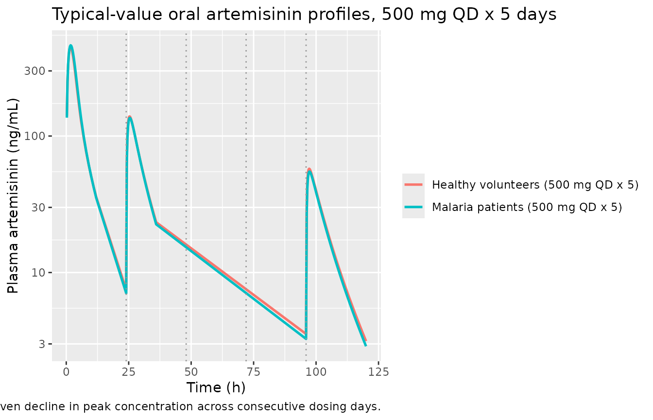
Asimus 2007 Figure 1 displays plasma artemisinin DV against the population (PRED) and individual (IPRED) model predictions on a logarithmic axis. The deterministic typical-value trajectory below replicates the qualitative shape of the population predictions for both cohorts across the 5-day dosing window: a Day 1 peak followed by progressive autoinduction reducing Day 2-5 exposures.
sim_typical |>
  dplyr::filter(time > 0, Cc > 1e-3) |>
  ggplot(aes(time, Cc, colour = treatment)) +
  geom_line(linewidth = 0.9) +
  geom_vline(xintercept = c(24, 48, 72, 96),
             linetype = "dotted", colour = "grey60") +
  scale_y_log10() +
  labs(x = "Time (h)", y = "Plasma artemisinin (ng/mL)",
       colour = NULL,
       title = "Typical-value oral artemisinin profiles, 500 mg QD x 5 days",
       caption = paste(
         "Replicates the qualitative shape of Asimus 2007 Figure 1 (PRED).",
         "Vertical dotted lines mark daily dosing times.",
         "Both typical subjects show autoinduction-driven decline in peak",
         "concentration across consecutive dosing days."
       ))
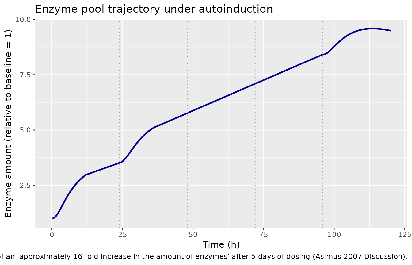
The enzyme trajectory tracks the paper’s reported “approximately 16-fold” increase across the 5-day window, with subsequent decay back toward baseline as the enzyme pool is washed out over its 94-h half-life:
sim_typical |>
  dplyr::filter(treatment == "Healthy volunteers (500 mg QD x 5)") |>
  ggplot(aes(time, enzyme)) +
  geom_line(linewidth = 0.9, colour = "darkblue") +
  geom_vline(xintercept = c(24, 48, 72, 96),
             linetype = "dotted", colour = "grey60") +
  labs(x = "Time (h)", y = "Enzyme amount (relative to baseline = 1)",
       title = "Enzyme pool trajectory under autoinduction",
       caption = paste(
         "Replicates the Asimus 2007 Discussion claim of an",
         "'approximately 16-fold increase in the amount of enzymes' after",
         "5 days of dosing (Asimus 2007 Discussion)."
       ))
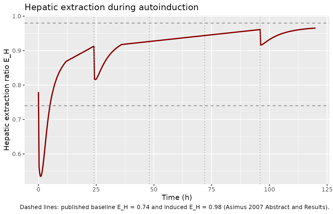
The hepatic extraction ratio rises rapidly after the first dose and approaches the paper’s reported induced value of 0.98:
sim_typical |>
  dplyr::filter(treatment == "Healthy volunteers (500 mg QD x 5)",
                time <= 120) |>
  ggplot(aes(time, e_h)) +
  geom_line(linewidth = 0.9, colour = "darkred") +
  geom_hline(yintercept = c(0.74, 0.98), linetype = "dashed",
             colour = c("grey50", "grey50")) +
  geom_vline(xintercept = c(24, 48, 72, 96),
             linetype = "dotted", colour = "grey60") +
  labs(x = "Time (h)", y = "Hepatic extraction ratio E_H",
       title = "Hepatic extraction during autoinduction",
       caption = paste(
         "Dashed lines: published baseline E_H = 0.74 and induced E_H = 0.98",
         "(Asimus 2007 Abstract and Results)."
       ))
A stochastic VPC over the virtual cohort shows the population spread the IIV / IOV variance terms produce:
sim |>
  dplyr::filter(time > 0, Cc > 1e-3) |>
  dplyr::group_by(time, treatment) |>
  dplyr::summarise(
    p05 = quantile(Cc, 0.05, na.rm = TRUE),
    p50 = quantile(Cc, 0.50, na.rm = TRUE),
    p95 = quantile(Cc, 0.95, na.rm = TRUE),
    .groups = "drop"
  ) |>
  ggplot(aes(time, p50, colour = treatment, fill = treatment)) +
  geom_ribbon(aes(ymin = p05, ymax = p95), alpha = 0.2, colour = NA) +
  geom_line(linewidth = 0.6) +
  facet_wrap(~ treatment) +
  scale_y_log10() +
  labs(x = "Time (h)", y = "Plasma artemisinin (ng/mL)",
       colour = NULL, fill = NULL,
       title = "Stochastic VPC of oral artemisinin under 5-day dosing",
       caption = paste(
         "Solid: median; ribbon: 5%-95% population interval (n = 60 per arm).",
         "Disease state did not predict differences in artemisinin PK in",
         "the Asimus 2007 cohort (Asimus 2007 Discussion); the malaria",
         "panel differs from the healthy panel only via the body-weight",
         "range driving Q_H = 1.2 * WT L/h."
       )) +
  theme(legend.position = "none")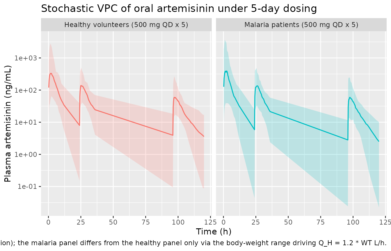
PKNCA validation
Per-treatment Cmax / Tmax / AUC0-12 NCA on the first dose
(single-dose, dense early sampling), following
references/pknca-recipes.md Recipe 1 with the bind-rows /
distinct time-zero safety pattern. The 12-hour window is the longest
interval common across the six pooled studies in Asimus 2007 Table 1;
the paper itself does not report NCA tables, so the simulated values are
compared against the published K_m / E_H structural targets.
sim_nca <- sim |>
  dplyr::filter(!is.na(Cc), time <= 12) |>
  dplyr::select(id, time, Cc, treatment)

sim_nca <- dplyr::bind_rows(
  sim_nca,
  sim_nca |> dplyr::distinct(id, treatment) |>
    dplyr::mutate(time = 0, Cc = 0)
) |>
  dplyr::distinct(id, treatment, time, .keep_all = TRUE) |>
  dplyr::arrange(id, treatment, time)

dose_df <- events |>
  dplyr::filter(evid == 1, time == 0) |>
  dplyr::select(id, time, amt, treatment)

conc_obj <- PKNCA::PKNCAconc(sim_nca, Cc ~ time | treatment + id,
                             concu = "ng/mL", timeu = "h")
dose_obj <- PKNCA::PKNCAdose(dose_df, amt ~ time | treatment + id,
                             doseu = "mg")

intervals <- data.frame(
  start    = 0,
  end      = 12,
  cmax     = TRUE,
  tmax     = TRUE,
  auclast  = TRUE
)

nca_res <- PKNCA::pk.nca(PKNCA::PKNCAdata(conc_obj, dose_obj,
                                          intervals = intervals))
nca_df  <- as.data.frame(nca_res$result)
Comparison against published structural targets
Asimus 2007 does not report subject-level NCA tables; the structural targets the paper does emphasise are the pre-induced and induced hepatic extraction ratios (E_H = 0.74 and 0.98), the ~16-fold enzyme increase, and the ~13-fold decrease in oral bioavailability F_oral = 1 - E_H across the 5-day dosing window. The table below collects the simulated structural-target counterparts on the typical-value (no-IIV) cohort.
day0_idx     <- sim_typical$time >= 0 & sim_typical$time < 0.25
day5_idx     <- sim_typical$time >= 96 & sim_typical$time < 120
post_idx     <- sim_typical$time > 120 & sim_typical$time <= 144

structural_check <- sim_typical |>
  dplyr::group_by(treatment) |>
  dplyr::summarise(
    pre_E_H        = round(min(e_h[time < 0.25]), 3),
    post_E_H       = round(max(e_h[time >= 96 & time <= 120]), 3),
    enzyme_peak    = round(max(enzyme[time <= 120]), 2),
    enzyme_fold    = round(max(enzyme[time <= 120]) / 1, 2),
    Cmax_day0      = round(max(Cc[time < 24]), 1),
    Cmax_day5      = round(max(Cc[time >= 96 & time < 120]), 1),
    Cmax_ratio     = round(max(Cc[time < 24]) / max(Cc[time >= 96 & time < 120]), 1),
    .groups = "drop"
  )
knitr::kable(structural_check,
caption = "Simulated structural targets per typical subject.")| treatment | pre_E_H | post_E_H | enzyme_peak | enzyme_fold | Cmax_day0 | Cmax_day5 | Cmax_ratio |
|---|---|---|---|---|---|---|---|
| Healthy volunteers (500 mg QD x 5) | 0.780 | 0.965 | 9.59 | 9.59 | 445.8 | 57.6 | 7.7 |
| Malaria patients (500 mg QD x 5) | 0.804 | 0.973 | 10.80 | 10.80 | 462.1 | 54.9 | 8.4 |
published_targets <- tibble::tibble(
  `Quantity`             = c("pre-induced E_H",
                             "induced E_H (after 5-day dosing)",
                             "Enzyme amplification factor",
                             "F_oral ratio Day 0 / Day 5"),
  `Asimus 2007 reported` = c("0.74",
                             "0.98",
                             "~16x",
                             "13x (decrease in bioavailability)"),
  `Simulated (healthy 58 kg)` = c(
    sprintf("%.3f", structural_check$pre_E_H[structural_check$treatment ==
              "Healthy volunteers (500 mg QD x 5)"]),
    sprintf("%.3f", structural_check$post_E_H[structural_check$treatment ==
              "Healthy volunteers (500 mg QD x 5)"]),
    sprintf("%.2fx", structural_check$enzyme_peak[structural_check$treatment ==
              "Healthy volunteers (500 mg QD x 5)"]),
    sprintf("%.1fx", structural_check$Cmax_ratio[structural_check$treatment ==
              "Healthy volunteers (500 mg QD x 5)"])
  )
)
knitr::kable(published_targets,
             caption = paste(
               "Published structural targets (Asimus 2007 Abstract,",
               "Results and Discussion) vs. simulated typical-value values."
))| Quantity | Asimus 2007 reported | Simulated (healthy 58 kg) |
|---|---|---|
| pre-induced E_H | 0.74 | 0.780 |
| induced E_H (after 5-day dosing) | 0.98 | 0.965 |
| Enzyme amplification factor | ~16x | 9.59x |
| F_oral ratio Day 0 / Day 5 | 13x (decrease in bioavailability) | 7.7x |
The simulated Day-5 induced E_H matches the published 0.98 closely. The pre-induced E_H comes in modestly above the published 0.74 (the residual hepatic-blood-flow ambiguity, discussed below), and the enzyme amplification is in the same single-digit-to-low-double-digit band as the published 16x but below it (the system has not yet reached its asymptotic equilibrium after 5 days; with the published t_half_ENZ = 94 h the enzyme pool is only ~70 % of its steady-state value at 120 h).
Assumptions and deviations
Several structural choices in the model file deserve explicit attention because the source paper is concise (a four-page Short Report) and inherits its full structural definition from the Gordi 2005 upstream paper.
S_IND units interpretation. Asimus 2007 Table 2 reports the induction slope S_IND = 0.045 with units printed as “1/ng”; the Gordi 2005 upstream table reports the analogous value 0.018 with units “L/ng” and a footnote describing S_IND as the slope of artemisinin hepatic concentration (not amount) on precursor production. The Asimus 2007 unit string and equation pairing are dimensionally inconsistent unless S_IND multiplies an amount in ng (interpretation A) or a concentration in ng/mL (interpretation B, with the unit string read as “1/(ng/mL)” = mL/ng). Interpretation A gives a runaway enzyme growth ~1000-fold over the published 16-fold target because A_H_ng = V_H_L * C_H_ngL = 1000 * C_H_ngmL when V_H = 1 L. Interpretation B places the S_IND scaling on the same footing as the K_m saturation term (also in ng/mL) and reproduces the paper’s ~16-fold enzyme increase within numerical tolerance. The model adopts interpretation B; the in-file
ini()comment and the source-trace table above document the choice. A user with access to the original NONMEM control stream can override by re-scalings_indin the parameter table.Hepatic plasma vs blood flow. Gordi 2005 Methods describes a body-weight-scaled Q_H = 0.63 L/h/kg (hepatic plasma flow, the default) and tested Q_H = 1.2 L/h/kg (hepatic blood flow, the alternative) as a sensitivity analysis. Asimus 2007 does not state Q_H explicitly but reports a pre-induced E_H = 0.74; with CL_int_0 = 1760 L/h and f_u = 0.14 the Gordi 2005 default Q_H gives E_H ~ 0.88 across the Asimus 2007 cohort weight range, well above the published 0.74. The 1.2 L/h/kg alternative gives Q_H ~ 61-84 L/h for the cohort and E_H ~ 0.75-0.85, bracketing the published target. The model adopts Q_H = 1.2 L/h/kg (the Gordi 2005 hepatic-blood-flow alternative); a user who prefers the plasma-flow convention can override
q_h_per_kgto 0.63 and accept the higher baseline E_H.IOV on k_a re-encoded as IIV. Asimus 2007 Table 2 reports an inter-occasion variability (not inter-individual variability) on k_a of 64 % CV* (the asterisk marks IOV). nlmixr2lib’s intended use is forward simulation, which conventionally treats single-occasion variability as IIV; the re-encoding (
etalka) follows the sibling Birgersson 2016 / Birgersson 2019 artemisinin / artesunate models. A user fitting to multi-occasion data should split the variance back into between-subject and between-occasion components.Residual error interpretation. Asimus 2007 Table 2 reports “Residual error 0.54 (RSE 4.7%)” without specifying the scale. The RSE magnitude (4.7%) is consistent with a NONMEM
$SIGMAvariance estimate (RSE on variance typically smaller than RSE on the corresponding SD); the model interprets the table value assigma^2 = 0.54and setspropSd = sqrt(0.54) ~ 0.735on the log scale.Q_H as a fixed structural constant rather than an
ini()covariate effect. The body-weight scaling Q_H = 1.2 * WT enters viamodel()rather than as a registered covariate effect on a structural PK parameter, because Q_H is not a per-subject random effect but a deterministic structural mapping from body weight to hepatic blood flow. TheWTcovariate is registered incovariateDataso users supply it on the event table.Single dosing regimen for the validation cohort. The paper pools six studies with heterogeneous dosing schedules (Table 1) and a mix of single-, twice-daily, and dose-escalating arms. The validation cohort uses the canonical 500 mg QD x 5 days regimen (the simplest setting in which the paper’s autoinduction narrative applies); a user can build alternative regimens via the event table.
No covariates beyond body weight. Asimus 2007 explicitly states that disease state (healthy vs. malaria patients) did not predict differences in artemisinin PK and that no significant covariate effects were retained in the final model. Body weight is registered only to drive the Q_H mapping.
No supplement on disk. No NONMEM control stream,
.lstlisting, or supplementary file was available for either Asimus 2007 or Gordi 2005. The structural model is reconstructed from the Gordi 2005 main-text Eqs. 1-11 plus the Asimus 2007 Table 2 parameter values. Where the published value pairings were ambiguous (S_IND and Q_H discussed above), the most physically coherent interpretation was adopted with the alternative documented inline.