Edoxaban and metabolite M4 (Jonsson 2015)
Source:vignettes/articles/Jonsson_2015_edoxaban.Rmd
Jonsson_2015_edoxaban.RmdModel and source
- Citation: Jonsson S., Simonsson U. S. H., Miller R., Karlsson M. O. (2015). Population pharmacokinetics of edoxaban and its main metabolite in a dedicated renal impairment study. The Journal of Clinical Pharmacology 55(11):1268-1279. doi:10.1002/jcph.541.
- Description: Joint parent plus metabolite population PK model for edoxaban and its main metabolite M4 in adults with normal kidney function through severe renal impairment, from a dedicated renal impairment study. Edoxaban disposition is two-compartment with Savic 2007 analytical transit-compartment absorption (non-integer NN, with the absorption rate constant constrained equal to the transit rate constant ktr) and absolute oral bioavailability estimated on the logit scale; edoxaban clearance is split into a renal arm that is linear in creatinine clearance and drives a urinary-excretion compartment, and a non-renal arm that is assumed to form all of the M4 metabolite. M4 is described by a one-compartment model with first-order formation. Fixed allometric body-weight scaling (0.75 on all clearance terms that are not a function of kidney function, 1 on all volumes) is applied around a 70 kg reference subject.
- Article: J Clin Pharmacol 2015;55(11):1268-1279
Edoxaban is an oral direct factor Xa inhibitor. This model was
developed on a dedicated renal impairment study and describes edoxaban
plasma concentrations, edoxaban urinary excretion, and plasma
concentrations of M4, its main human metabolite, simultaneously. Because
urine data allowed renal clearance (rather than apparent renal clearance
CLR/F) to be estimated, and because renal excretion
contributes about half of total clearance, the analysis was able to
estimate absolute oral bioavailability without an
intravenous reference arm.
This extraction was prepared from the published article and its
supplement together with material supplied directly by the first author
(Siv Jonsson, Uppsala University): the NONMEM control stream of the
final run (run164-share.mod), the analysis dataset, and its
data specification. The control stream is the authoritative record of
the model structure; all parameter values below come
from the paper’s Table 1, because a control stream’s $THETA
/ $OMEGA / $SIGMA blocks hold initial, not
final, estimates. The clearest illustration is the creatinine-clearance
slope: the control stream carries an initial value of 0.0862453 whereas
the final estimate in Table 1 is 0.109. Neither the dataset nor the
control stream is redistributed with this package.
Structure
                       transit chain (Savic 2007, non-integer NN)
  15 mg oral dose  ->  gamma-density input  ->  depot --ktr--> central <--Q--> peripheral1
                                                                 |  |
                                                     CLR (= f(CLcr))  CLNR
                                                                 |        |
urine central_m4 --CLM4--> out-
Edoxaban: two compartments (
central,peripheral1) with transit-compartment absorption. The absorption rate constant was not separately identifiable, so the depot empties intocentralat the same ratektr = (NN + 1) / MTTthat governs transit. -
Clearance split:
CL = CLNR + CLR. The renal armCLRis a linear function of creatinine clearance and drives theurinecompartment; the non-renal armCLNRis assumed to form all of the M4 metabolite. -
M4: one compartment (
central_m4) with first-order formation fromCLNR, in molar units so the 1:1 stoichiometry is exact.
Because the fraction of edoxaban converted to M4 was not
identifiable, the model assumes fm,M4 = 1 - fe = CLNR/CL.
CLM4 and VM4 are therefore
apparent values, overestimated relative to the true
ones by 1/fm,M4.
Population
Thirty-two subjects each received a single oral 15 mg edoxaban tablet in an open-label parallel-group study, allocated by Cockcroft-Gault creatinine clearance to four groups of eight: normal kidney function (CLcr > 80 mL/min), mild (50 <= CLcr <= 80), moderate (30 <= CLcr < 50) and severe renal impairment (CLcr < 30, not on dialysis). Group mean (range) CLcr was 94.6 (83.0-123.0), 64.7 (54.0-77.0), 42.0 (33.0-49.0) and 21.8 (14.0-27.0) mL/min; body weight was 74.4 (58.9-89.4), 76.5 (60.3-91.0), 78.6 (58.0-90.0) and 71.7 (56.0-95.0) kg; age was 50.1 (30.0-64.0), 56.8 (38.0-65.0), 50.8 (30.8-67.0) and 53.1 (41.0-63.0) years. The male/female split was 6/2, 4/4, 5/3 and 3/5, i.e. 43.8% female overall, and all subjects were White (Jonsson 2015 Results, “Data”).
The analysis used 360 edoxaban plasma, 159 edoxaban urine and 294 M4 plasma concentrations. A fifth study group of subjects with end-stage renal disease on peritoneal dialysis was enrolled but excluded from this analysis, so the model should not be extrapolated to dialysis patients.
The same information is available programmatically:
str(readModelDb("Jonsson_2015_edoxaban")()$population, max.level = 1)
#> List of 14
#>  $ species       : chr "human"
#>  $ n_subjects    : int 32
#>  $ n_studies     : int 1
#>  $ age_range     : chr "30.0-67.0 years across the four renal-function groups (study eligibility 18-75 years)"
#>  $ age_median    : chr "group means 50.1, 56.8, 50.8 and 53.1 years for normal, mild, moderate and severe renal impairment"
#>  $ weight_range  : chr "56.0-95.0 kg across the four renal-function groups (study eligibility 55-110 kg)"
#>  $ weight_median : chr "group means 74.4, 76.5, 78.6 and 71.7 kg for normal, mild, moderate and severe renal impairment"
#>  $ sex_female_pct: num 43.8
#>  $ race_ethnicity: Named num 100
#>   ..- attr(*, "names")= chr "White"
#>  $ disease_state : chr "Open-label, parallel-group, single-dose dedicated renal impairment study in subjects with varying degrees of ki"| __truncated__
#>  $ dose_range    : chr "Single oral 15 mg edoxaban tablet (27372 nmol) taken after a light breakfast with 240 mL water"
#>  $ regions       : chr "Not stated in the publication"
#>  $ renal_function: chr "Full spectrum from normal kidney function to severe renal impairment. A fifth study group of subjects with end-"| __truncated__
#>  $ notes         : chr "Baseline demographics from Jonsson 2015 Results 'Data'. Sex distribution (male/female) was 6/2, 4/4, 5/3 and 3/"| __truncated__
Source trace
Every ini() entry in
inst/modeldb/specificDrugs/Jonsson_2015_edoxaban.R carries
an in-file comment naming its origin. They are collected here for
review. All values are from Table 1, “Estimate (%RSE)”
column unless noted.
| Equation / parameter | Value | Source location |
|---|---|---|
lmtt (MTT) |
0.731 h | Table 1, “Mean transit time (MTT), h” |
lnn (NN, fixed) |
8.08 | Table 1, “Number of transit compartments (NN)”; footnote c “not estimated … fixed” |
logitfdepot (F) |
0.723 | Table 1, “Absolute oral bioavailability (F)”; logit form from
control-stream $PK
PSI = LOG(TVF1/(1-TVF1))
|
lcl_nonren (CLNR) |
10.1 L/h | Table 1, “Nonrenal clearance (CLNR), L/h” |
lvc (Vc) |
95.4 L | Table 1, “Central volume of distribution (Vc), L” |
lvp (Vp) |
54.3 L | Table 1, “Peripheral volume of distribution (Vp), L” |
lq (Q) |
5.19 L/h | Table 1, “Intercompartmental clearance (Q), L/h” |
lcl_m4 (CLM4, apparent) |
113 L/h | Table 1, “Apparent clearance M4 (CLM4), L/h” |
lvc_m4 (VM4, apparent) |
78.1 L | Table 1, “Apparent volume of distribution M4 (VM4), L” |
lcl_renal (CLR at CLcr = 100) |
0.109 x 100 = 10.9 L/h | Table 1, “CLcr on CL (slopeCLcr)” = 0.109 L/h per mL/min; footnote d |
e_wt_cl_q (fixed) |
0.75 | Results, “exponents fixed to 1 and 3/4 for volume and clearance terms” |
e_wt_vc_vp (fixed) |
1 | Results, same sentence |
etalcl_nonren |
0.177^2 | Table 1, “CLNR, %CV” = 17.7 |
etalcl_renal |
0.271^2 | Table 1, “Renal clearance (CLR), %CV” = 27.1 |
etalvc |
0.165^2 | Table 1, “Vc, %CV” = 16.5 |
etalvp |
0.351^2 | Table 1, “Vp, %CV” = 35.1 |
etalmtt |
0.532^2 | Table 1, “MTT, %CV” = 53.2 |
etalnn (fixed) |
1.22^2 | Table 1, “NN, %CV” = 122; footnote c |
etalogitfdepot |
0.4149 | Table 1, “F” = 0.129 with footnote g (see below) |
etalcl_m4 + etalvc_m4 block |
0.498^2, r = 0.848, 0.425^2 | Table 1, “CLM4, %CV”, “Correlation CLM4-VM4”, “VM4, %CV” |
propSd |
0.154 | Table 1, “Proportional residual error, edoxaban plasma concentrations, %CV” = 15.4 |
propSd_m4 |
0.184 | Table 1, “Proportional residual error, M4 plasma concentrations, %CV” = 18.4 |
propSd_Aurine |
0.254 | Table 1, “Proportional residual error, edoxaban urine concentrations, %CV” = 25.4 |
CL = CLNR*(WT/70)^0.75 + slopeCLcr*CLcr |
n/a | Results, “Clearance for edoxaban was parameterized as follows”; Table 1 footnote d |
Vc = Vc,typ*(WT/70)^1,
Q = Q_typ*(WT/70)^0.75
|
n/a | Results, “Volume and other clearance parameters were parameterized as exemplified for Vc and Q” |
AUC = F*dose/CL,
AUC_M4 = F*fm*dose/CLM4
|
n/a | Methods, “Final Population PK Model Predictions” |
| transit input / depot ODEs | n/a | Control stream $DES DADT(1); Savic 2007
(Jonsson 2015 reference 20) |
Two back-transforms worth spelling out
IIV “%CV” is on the approximate SD scale. Table 1
labels the IIV column “%CV” (footnote f), but the values are
100 * sqrt(omega^2), not the exact log-normal
100 * sqrt(exp(omega^2) - 1). NN settles this
unambiguously, because its IIV was fixed and so cannot have moved
between the control stream and the final fit:
omega_nn <- 1.50033   # control stream: $OMEGA 1.50033 FIX
c(
  `approximate SD scale` = 100 * sqrt(omega_nn),
  `exact log-normal`     = 100 * sqrt(exp(omega_nn) - 1),
  `Table 1 reports`      = 122
)
#> approximate SD scale     exact log-normal      Table 1 reports
#>             122.4880             186.6325             122.0000
Footnote a corroborates this (“reported on the approximate standard
deviation scale”). Every variance in ini() is therefore
(%CV / 100)^2.
IIV on F is reported on the natural scale, not the logit scale. Footnote g states “Because of logit transformation, variability is standard deviation (SD) = F x (1-F) x vF”, so the tabulated 0.129 is a delta-method SD on the F scale. Inverting it recovers the logit-scale variance actually used:
f_typ <- 0.723
sd_logit <- 0.129 / (f_typ * (1 - f_typ))
c(`logit-scale SD` = sd_logit,
  `logit-scale variance (used in ini())` = sd_logit^2,
  `control-stream initial $OMEGA` = 0.446911)
#>                       logit-scale SD logit-scale variance (used in ini())
#>                            0.6441272                            0.4148999
#>        control-stream initial $OMEGA
#>                            0.4469110
Units and dosing
The original analysis ran entirely in molar units: doses in nmol and concentrations in nmol/L (nM). Jonsson 2015 Methods, “Data”: “By using concentrations in nM and dose amounts in nmol, the difference in molecular weights for edoxaban and M4 was taken into account.” Working in molar units is what makes the 1:1 metabolite formation term exact, so the packaged model keeps them.
MW_EDOXABAN <- 548.0                        # g/mol, edoxaban free base
mg_to_nmol  <- function(mg) mg / MW_EDOXABAN * 1e6
DOSE_15MG   <- mg_to_nmol(15)
c(`15 mg (nmol)` = DOSE_15MG, `30 mg` = mg_to_nmol(30), `60 mg` = mg_to_nmol(60))
#> 15 mg (nmol)        30 mg        60 mg
#>     27372.26     54744.53    109489.05
The molecular weight is not printed in the paper; 548.0 g/mol is the edoxaban free-base value and is confirmed by the author-supplied analysis dataset, whose molar dose column holds 27372.26 nmol for the 15 mg tablet (15/548.0 x 1e6 = 27372.26). It is used only to convert mg to nmol for display; no model parameter depends on it. Every validation target in this vignette is a clearance, a ratio, or a percentage, so all of them are independent of the molecular weight.
Virtual cohort
Individual data are not publicly available. The cohort below reproduces the four renal-function strata, sampling CLcr uniformly across each group’s observed range and body weight normally about each group’s observed mean, truncated to the study’s 55-110 kg eligibility window.
set.seed(20150541)

N_PER_GROUP <- 100L   # <= 200 per arm

groups <- tibble::tribble(
  ~renal_group,             ~crcl_lo, ~crcl_hi, ~wt_mean,
  "Normal (CLcr > 80)",         83.0,    123.0,     74.4,
  "Mild (50-80)",               54.0,     77.0,     76.5,
  "Moderate (30-50)",           33.0,     49.0,     78.6,
  "Severe (< 30)",              14.0,     27.0,     71.7
) |>
  mutate(renal_group = factor(renal_group, levels = renal_group))

# Study sampling schedule (Jonsson 2015 Methods, "Data"). The urine collection
# boundaries (4, 8, 12, 24, 48 h) are already members of this set, so the same
# grid serves the plasma and the urine endpoints.
OBS_TIMES   <- c(0, 0.5, 1, 2, 3, 4, 6, 8, 10, 12, 24, 36, 48, 72)
URINE_EDGES <- c(0, 4, 8, 12, 24, 48)

make_cohort <- function(n, crcl_lo, crcl_hi, wt_mean, renal_group, id_offset = 0L) {
  subj <- tibble(
    id          = id_offset + seq_len(n),
    renal_group = renal_group,
    CRCL        = runif(n, crcl_lo, crcl_hi),
    WT          = pmin(110, pmax(55, rnorm(n, wt_mean, 9)))
  )
  bind_rows(
    subj |> mutate(time = 0, evid = 1L, cmt = "depot", amt = DOSE_15MG,
                   dvid = NA_integer_),
    subj |> tidyr::crossing(time = OBS_TIMES) |>
      mutate(evid = 0L, cmt = "central", amt = NA_real_, dvid = 1L)
  ) |>
    arrange(id, time, desc(evid))
}

events <- bind_rows(
  lapply(seq_len(nrow(groups)), function(i) {
    make_cohort(
      n           = N_PER_GROUP,
      crcl_lo     = groups$crcl_lo[i],
      crcl_hi     = groups$crcl_hi[i],
      wt_mean     = groups$wt_mean[i],
      renal_group = groups$renal_group[i],
      id_offset   = (i - 1L) * N_PER_GROUP
    )
  })
)

# Disjoint IDs across cohorts are mandatory: rxSolve keys subjects on id, and
# duplicates silently merge into one subject receiving the summed dose.
stopifnot(!anyDuplicated(unique(events[, c("id", "time", "evid")])))
c(subjects = dplyr::n_distinct(events$id), rows = nrow(events))
#> subjects     rows
#>      400     6000
Observation rows use cmt = "central" (an actual ODE
state) together with dvid = 1L. This model has five ODE
states and three ~ endpoints, so rxode2 allocates endpoint
slots after the state slots; naming the state and supplying
dvid keeps the mapping unambiguous. rxode2 still returns
Cc, Cc_m4 and Aurine as columns
on those rows.
Simulation
mod <- readModelDb("Jonsson_2015_edoxaban")

sim <- rxode2::rxSolve(
  mod, events = events,
  keep = c("renal_group", "WT", "CRCL")
) |>
  as.data.frame() |>
  mutate(renal_group = factor(as.character(renal_group),
                              levels = levels(groups$renal_group)))
#> ℹ parameter labels from comments will be replaced by 'label()'

sim |> select(id, time, renal_group, WT, CRCL, Cc, Cc_m4, Aurine) |> head(4)
#>   id time        renal_group       WT     CRCL       Cc     Cc_m4    Aurine
#> 1  1  0.0 Normal (CLcr > 80) 70.01748 100.7516   0.0000  0.000000    0.0000
#> 2  1  0.5 Normal (CLcr > 80) 70.01748 100.7516 138.3141  3.008325  175.6683
#> 3  1  1.0 Normal (CLcr > 80) 70.01748 100.7516 165.0345 12.009390  854.7713
#> 4  1  2.0 Normal (CLcr > 80) 70.01748 100.7516 128.9651 18.629946 2056.3368
The typical-value model, used below for the deterministic replications:
mod_typical <- rxode2::zeroRe(mod)
#> ℹ parameter labels from comments will be replaced by 'label()'
# Solve the typical-value model for one covariate combination.
solve_typical <- function(crcl, wt = 70, dose = DOSE_15MG,
                          times = seq(0, 72, by = 0.25), ...) {
  ev <- bind_rows(
    tibble(id = 1L, time = 0, evid = 1L, cmt = "depot", amt = dose,
           dvid = NA_integer_),
    tibble(id = 1L, time = times, evid = 0L, cmt = "central",
           amt = NA_real_, dvid = 1L)
  ) |>
    mutate(WT = wt, CRCL = crcl) |>
    arrange(time, desc(evid))
  rxode2::rxSolve(mod_typical, ev, ...) |>
    as.data.frame() |>
    mutate(CRCL = crcl, WT = wt, dose = dose)
}
Replicate published figures
Figure 3 – predictive checks for the three measured entities
# Replicates Figure 3 of Jonsson 2015: edoxaban plasma, edoxaban urine and M4
# plasma versus time after dose, stratified by renal function.

# Urine is fitted by the authors as the amount excreted during each collection
# interval divided by that interval's volume. The packaged model carries the
# CUMULATIVE amount, so interval amounts come from differencing at the
# collection boundaries.
urine_intervals <- sim |>
  filter(time %in% URINE_EDGES) |>
  arrange(id, time) |>
  group_by(id, renal_group) |>
  mutate(interval_amt = Aurine - lag(Aurine),
         interval_end = time) |>
  ungroup() |>
  filter(!is.na(interval_amt))

plasma_long <- sim |>
  filter(time > 0) |>
  select(id, time, renal_group, Cc, Cc_m4) |>
  pivot_longer(c(Cc, Cc_m4), names_to = "entity", values_to = "value") |>
  mutate(entity = recode(entity,
                         Cc    = "Edoxaban plasma (nM)",
                         Cc_m4 = "M4 plasma (nM)"))

bind_rows(
  plasma_long,
  urine_intervals |>
    transmute(id, time = interval_end, renal_group,
              entity = "Edoxaban urine, amount per interval (nmol)",
              value = interval_amt)
) |>
  filter(value > 0) |>
  group_by(entity, renal_group, time) |>
  summarise(Q05 = quantile(value, 0.05), Q50 = median(value),
            Q95 = quantile(value, 0.95), .groups = "drop") |>
  ggplot(aes(time, Q50, colour = renal_group, fill = renal_group)) +
  geom_ribbon(aes(ymin = Q05, ymax = Q95), alpha = 0.15, colour = NA) +
  geom_line(linewidth = 0.7) +
  facet_wrap(~entity, ncol = 1, scales = "free_y") +
  scale_y_log10() +
  labs(x = "Time after dose (h)", y = NULL, colour = NULL, fill = NULL,
       title = "Figure 3 -- median and 5th-95th percentile by renal function",
       caption = "Replicates Figure 3 of Jonsson 2015.") +
  theme(legend.position = "bottom")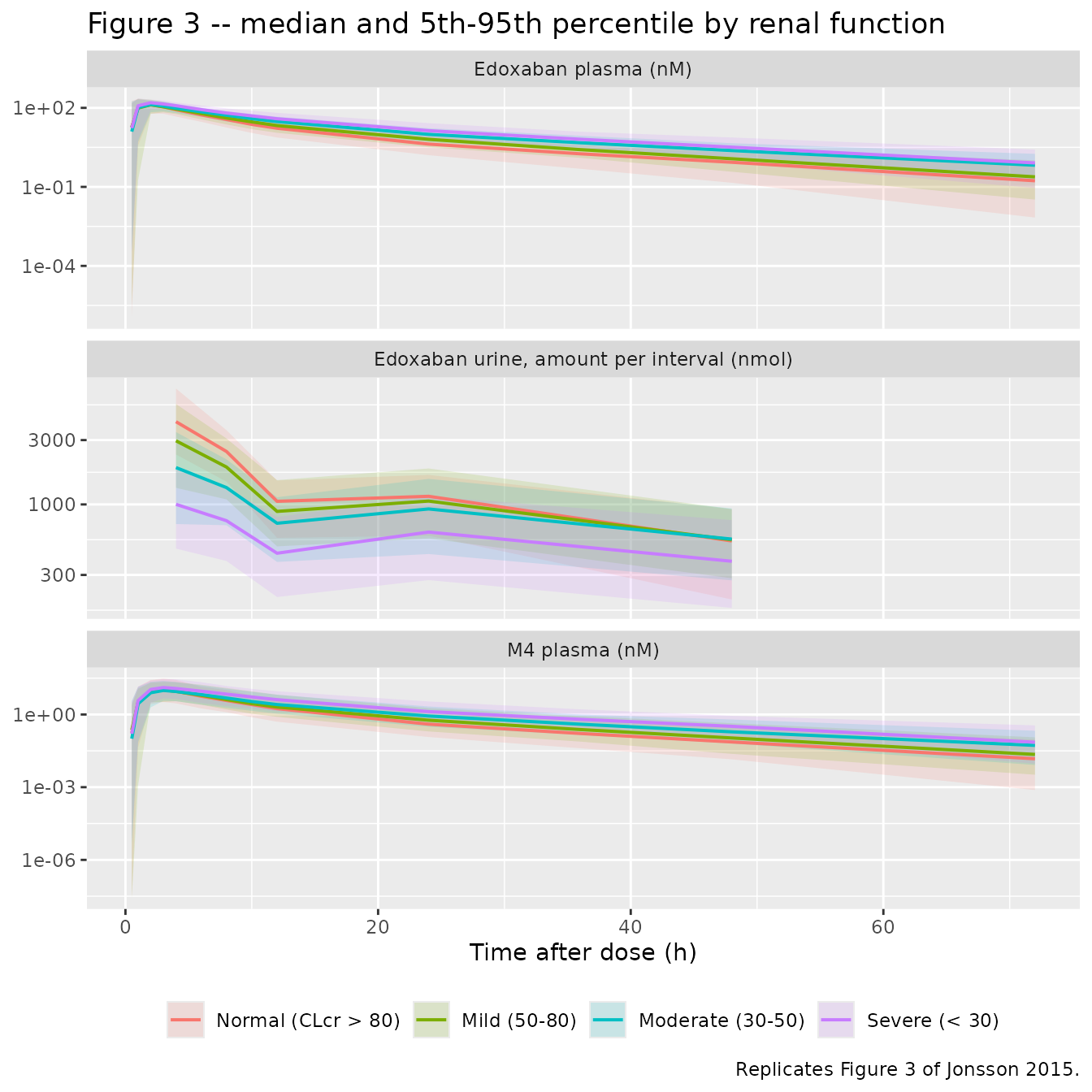
Exposure of both edoxaban and M4 rises as kidney function falls, and urinary excretion falls, as in the published figure.
Figure 4 – concentration ratio M4 / edoxaban
# Replicates Figure 4 of Jonsson 2015: concentration ratio versus time after
# dose (stratified by renal function) and versus CLcr (stratified by time).
ratios <- sim |>
  filter(time > 0, Cc > 0) |>
  mutate(ratio = Cc_m4 / Cc)

p_time <- ratios |>
  group_by(renal_group, time) |>
  summarise(Q50 = median(ratio), .groups = "drop") |>
  ggplot(aes(time, Q50, colour = renal_group)) +
  geom_line(linewidth = 0.7) +
  labs(x = "Time after dose (h)", y = "M4 / edoxaban", colour = NULL,
       title = "Concentration ratio vs time") +
  theme(legend.position = "bottom")

p_crcl <- ratios |>
  filter(time %in% c(2, 12, 24, 48)) |>
  ggplot(aes(CRCL, ratio)) +
  geom_point(alpha = 0.2, size = 0.6) +
  geom_smooth(method = "loess", formula = y ~ x, se = FALSE, linewidth = 0.7) +
  facet_wrap(~time, labeller = label_both) +
  labs(x = "CLcr (mL/min)", y = "M4 / edoxaban",
       title = "Concentration ratio vs CLcr")

p_time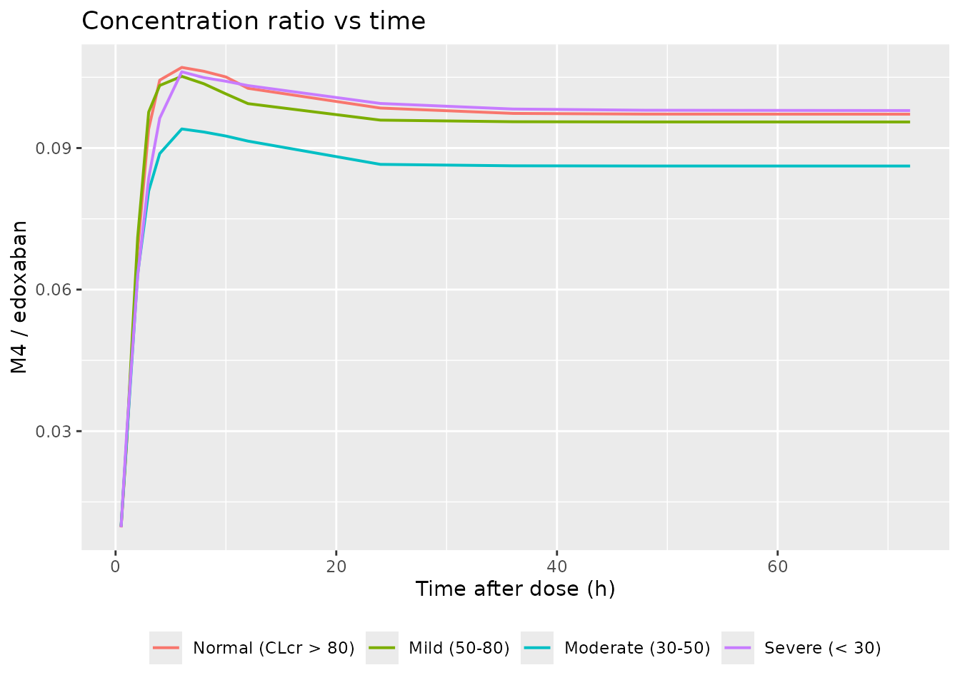
p_crcl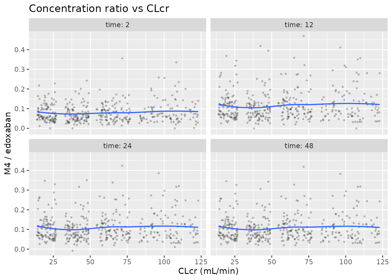
The ratio varies with time after dose because M4 formation is slower than edoxaban absorption, but is only weakly related to kidney function – the paper’s central conclusion.
Figure 5 – typical AUC and concentration ratio at steady state
# Replicates Figure 5 of Jonsson 2015: typical model-predicted steady-state AUC
# of edoxaban and M4 by body weight and CLcr for 30 and 60 mg once daily, and
# the predicted concentration ratio over one dosing interval.
#
# For a linear model the steady-state AUC over one dosing interval equals the
# single-dose AUC0-inf, so it is evaluated analytically here from the model's
# own parameter equations rather than by integrating to steady state.
auc_grid <- tidyr::crossing(
  WT   = c(60, 70, 90),
  CRCL = seq(15, 105, by = 5),
  dose_mg = c(30, 60)
) |>
  mutate(
    cl_nonren = 10.1 * (WT / 70)^0.75,
    cl_renal  = 0.109 * CRCL,
    cl        = cl_nonren + cl_renal,
    cl_m4     = 113 * (WT / 70)^0.75,
    fm        = cl_nonren / cl,
    AUC_edox  = 0.723 * mg_to_nmol(dose_mg) / cl,
    AUC_m4    = 0.723 * fm * mg_to_nmol(dose_mg) / cl_m4,
    ratio     = AUC_m4 / AUC_edox
  )

auc_grid |>
  select(WT, CRCL, dose_mg, AUC_edox, AUC_m4) |>
  pivot_longer(c(AUC_edox, AUC_m4), names_to = "entity", values_to = "AUC") |>
  mutate(entity  = recode(entity, AUC_edox = "Edoxaban", AUC_m4 = "M4"),
         dose_lb = paste0(dose_mg, " mg once daily")) |>
  ggplot(aes(CRCL, AUC, colour = factor(WT))) +
  geom_line(linewidth = 0.7) +
  facet_grid(entity ~ dose_lb, scales = "free_y") +
  labs(x = "CLcr (mL/min)", y = "Steady-state AUC over one interval (nM*h)",
       colour = "Body weight (kg)",
       title = "Figure 5 (top) -- typical steady-state AUC",
       caption = "Replicates Figure 5 (top) of Jonsson 2015.") +
  theme(legend.position = "bottom")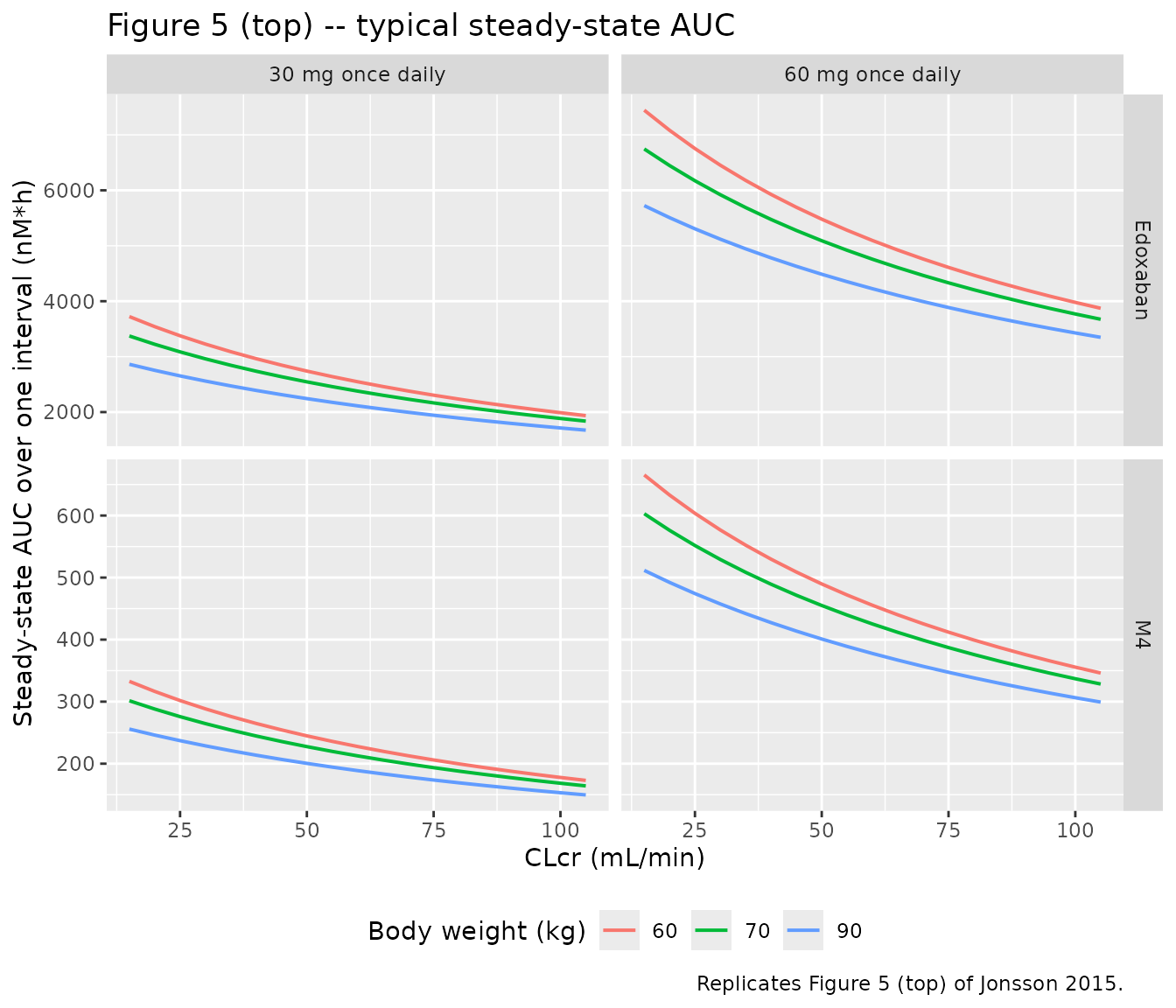
The paper states the AUC ratio is constant across CLcr, body weight
and dose. That is a structural consequence of the parameterisation:
CLNR and CLM4 carry the same
allometric exponent, so
AUC_M4 / AUC_edox = (F*fm*dose/CLM4) / (F*dose/CL) = fm*CL/CLM4 = CLNR/CLM4,
which contains neither weight nor CLcr. The simulation confirms the invariance:
c(`distinct AUC ratios over the whole grid` = dplyr::n_distinct(round(auc_grid$ratio, 10)),
  `ratio value`                             = unique(round(auc_grid$ratio, 5)),
  `CLNR / CLM4`                             = round(10.1 / 113, 5),
  `paper reports`                           = 0.085)
#> distinct AUC ratios over the whole grid                             ratio value
#>                                 1.00000                                 0.08938
#>                             CLNR / CLM4                           paper reports
#>                                 0.08938                                 0.08500
# Replicates Figure 5 (bottom): concentration ratio over one dosing interval at
# steady state, for combinations of body weight and CLcr.
ss_ratio <- bind_rows(lapply(
  split(tidyr::crossing(WT = c(60, 90), CRCL = c(20, 50, 100)),
        seq_len(6)),
  function(g) {
    # Dose 60 mg once daily for 14 days, then follow one interval.
    ev <- bind_rows(
      tibble(id = 1L, time = seq(0, 13 * 24, by = 24), evid = 1L,
             cmt = "depot", amt = mg_to_nmol(60), dvid = NA_integer_),
      tibble(id = 1L, time = 13 * 24 + seq(0, 24, by = 0.25), evid = 0L,
             cmt = "central", amt = NA_real_, dvid = 1L)
    ) |>
      mutate(WT = g$WT, CRCL = g$CRCL) |>
      arrange(time, desc(evid))
    rxode2::rxSolve(mod_typical, ev) |>
      as.data.frame() |>
      mutate(WT = g$WT, CRCL = g$CRCL, tad = time - 13 * 24)
  }
))
#> ℹ omega/sigma items treated as zero: 'etalcl_nonren', 'etalcl_renal', 'etalvc', 'etalvp', 'etalmtt', 'etalnn', 'etalogitfdepot', 'etalcl_m4', 'etalvc_m4'
#> ℹ omega/sigma items treated as zero: 'etalcl_nonren', 'etalcl_renal', 'etalvc', 'etalvp', 'etalmtt', 'etalnn', 'etalogitfdepot', 'etalcl_m4', 'etalvc_m4'
#> ℹ omega/sigma items treated as zero: 'etalcl_nonren', 'etalcl_renal', 'etalvc', 'etalvp', 'etalmtt', 'etalnn', 'etalogitfdepot', 'etalcl_m4', 'etalvc_m4'
#> ℹ omega/sigma items treated as zero: 'etalcl_nonren', 'etalcl_renal', 'etalvc', 'etalvp', 'etalmtt', 'etalnn', 'etalogitfdepot', 'etalcl_m4', 'etalvc_m4'
#> ℹ omega/sigma items treated as zero: 'etalcl_nonren', 'etalcl_renal', 'etalvc', 'etalvp', 'etalmtt', 'etalnn', 'etalogitfdepot', 'etalcl_m4', 'etalvc_m4'
#> ℹ omega/sigma items treated as zero: 'etalcl_nonren', 'etalcl_renal', 'etalvc', 'etalvp', 'etalmtt', 'etalnn', 'etalogitfdepot', 'etalcl_m4', 'etalvc_m4'

ss_ratio |>
  filter(tad > 0) |>
  mutate(label = paste0(WT, " kg, CLcr ", CRCL)) |>
  ggplot(aes(tad, Cc_m4 / Cc, colour = label)) +
  geom_line(linewidth = 0.7) +
  labs(x = "Time after dose within the interval (h)", y = "M4 / edoxaban",
       colour = NULL,
       title = "Figure 5 (bottom) -- steady-state concentration ratio",
       caption = "Replicates Figure 5 (bottom) of Jonsson 2015.") +
  theme(legend.position = "bottom")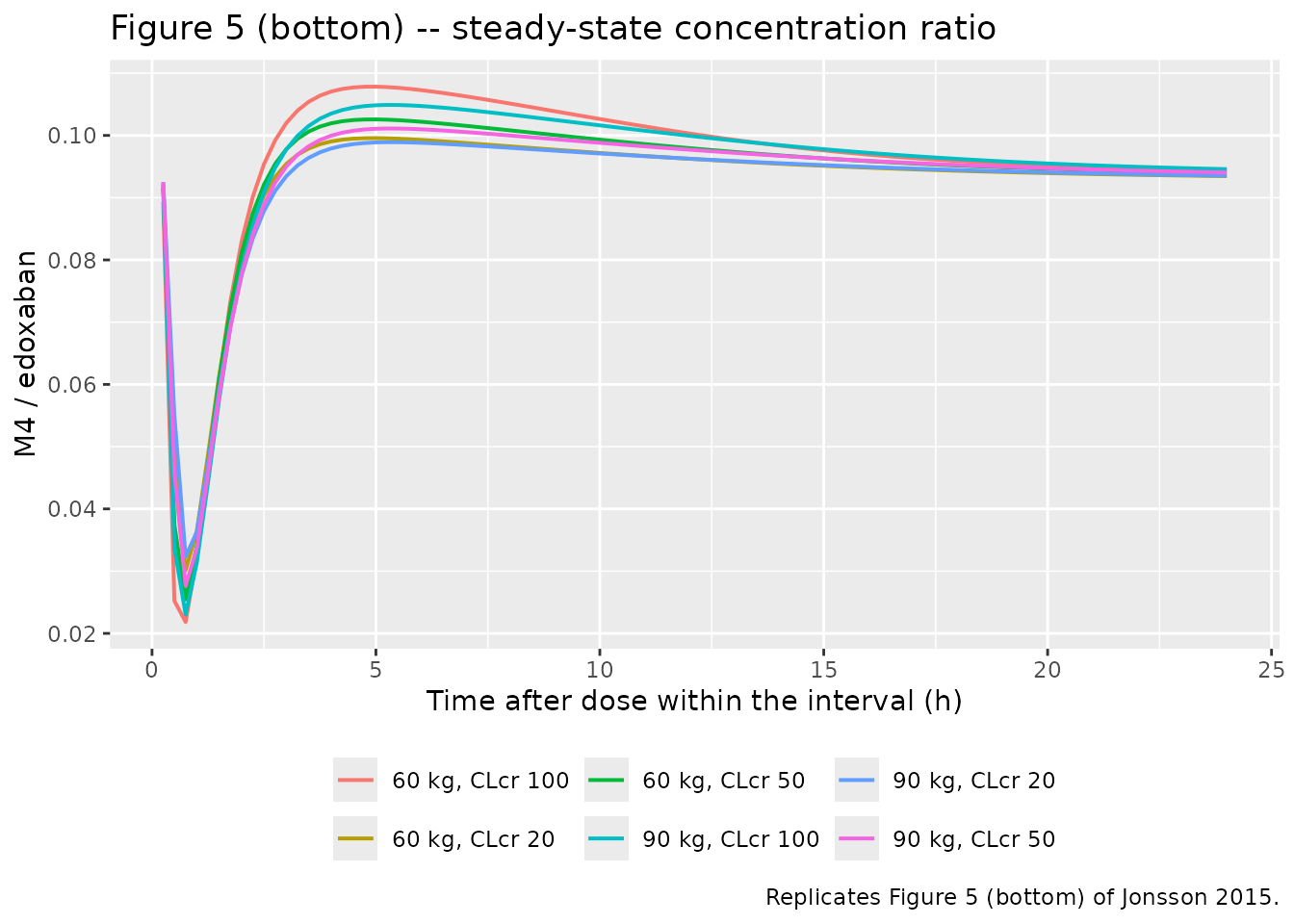
ss_ratio |>
  filter(tad > 0) |>
  summarise(`min ratio` = min(Cc_m4 / Cc), `max ratio` = max(Cc_m4 / Cc))
#>    min ratio max ratio
#> 1 0.02182666 0.1078331
The paper describes the ratio as varying “approximately between 0.02 and 0.1” over a dosing interval, with little influence of kidney function or body weight.
PKNCA validation
Edoxaban plasma, by renal-function group
# Use only !is.na(Cc): a `time > 0` or `Cc > 0` filter would drop the time-zero
# row that PKNCA needs to anchor AUC0-*.
conc_edox <- sim |>
  filter(!is.na(Cc)) |>
  select(id, time, Cc, renal_group)

# Guarantee a time = 0 row per subject; pre-dose Cc = 0 is correct for an
# extravascular dose.
conc_edox <- bind_rows(
  conc_edox,
  conc_edox |> distinct(id, renal_group) |> mutate(time = 0, Cc = 0)
) |>
  distinct(id, renal_group, time, .keep_all = TRUE) |>
  arrange(id, renal_group, time)

dose_df <- events |>
  filter(evid == 1) |>
  select(id, time, amt) |>
  left_join(distinct(sim, id, renal_group), by = "id")

intervals <- data.frame(
  start = 0, end = Inf,
  cmax = TRUE, tmax = TRUE, aucinf.obs = TRUE, half.life = TRUE, cl.obs = TRUE
)

nca_edox <- PKNCA::pk.nca(PKNCA::PKNCAdata(
  PKNCA::PKNCAconc(conc_edox, Cc ~ time | renal_group + id),
  PKNCA::PKNCAdose(dose_df,   amt ~ time | renal_group + id),
  intervals = intervals
))
#> Warning in assert_conc(conc, any_missing_conc = any_missing_conc): Negative
#> concentrations found
#> Warning: Too few points for half-life calculation (min.hl.points=3 with only 0
#> points)
#> Warning in assert_conc(conc = conc): Negative concentrations found
#> Warning in assert_conc(conc, any_missing_conc = any_missing_conc): Negative
#> concentrations found
#> Warning in assert_conc(conc, any_missing_conc = any_missing_conc): Negative
#> concentrations found
#> Warning in assert_conc(conc, any_missing_conc = any_missing_conc): Negative
#> concentrations found
#> Warning in assert_conc(conc, any_missing_conc = any_missing_conc): Negative
#> concentrations found
#> Warning in assert_conc(conc, any_missing_conc = any_missing_conc): Negative
#> concentrations found
#> Warning in log(data$conc): NaNs produced
#> Warning: Too few points for half-life calculation (min.hl.points=3 with only 1
#> points)
#> Warning in assert_conc(conc, any_missing_conc = any_missing_conc): Negative
#> concentrations found
#> Warning in log(conc.2/conc.1): NaNs produced

as.data.frame(nca_edox) |>
  filter(PPTESTCD %in% c("cmax", "tmax", "aucinf.obs", "half.life", "cl.obs")) |>
  group_by(renal_group, PPTESTCD) |>
  summarise(median = median(PPORRES, na.rm = TRUE), .groups = "drop") |>
  pivot_wider(names_from = PPTESTCD, values_from = median) |>
  relocate(renal_group, cmax, tmax, aucinf.obs, half.life, cl.obs) |>
  rename("Renal function"      = renal_group,
         "Cmax (nM)"           = cmax,
         "Tmax (h)"            = tmax,
         "AUC0-inf (nM*h)"     = aucinf.obs,
         "t1/2 (h)"            = half.life,
         "CL/F (L/h)"          = cl.obs) |>
  knitr::kable(digits = c(0, 1, 2, 0, 2, 2),
caption = "Median simulated edoxaban NCA by renal-function group (single 15 mg oral dose).")| Renal function | Cmax (nM) | Tmax (h) | AUC0-inf (nM*h) | t1/2 (h) | CL/F (L/h) |
|---|---|---|---|---|---|
| Normal (CLcr > 80) | 147.4 | 2 | 915 | 10.55 | 29.78 |
| Mild (50-80) | 144.8 | 2 | 997 | 10.40 | 27.46 |
| Moderate (30-50) | 144.0 | 2 | 1234 | 12.36 | 22.19 |
| Severe (< 30) | 169.2 | 2 | 1568 | 11.85 | 17.45 |
Comparison against the published CL/F predictions
The paper reports typical model-predicted CL/F at four
specific creatinine clearances (Discussion: “The typical CL/F at a CLcr
of 22, 42, 68, and 95 mL/min was estimated as 17.3, 20.3, 24.2, and 28.3
L/h”). This is the sharpest available check on the clearance
parameterisation, so it is reproduced from the typical-value model.
clf_sim <- bind_rows(lapply(c(22, 42, 68, 95), function(cc) {
  solve_typical(cc, times = c(0, seq(0.1, 72, by = 0.1))) |>
    mutate(id = cc, crcl_group = paste0("CLcr ", cc, " mL/min"))
}))
#> ℹ omega/sigma items treated as zero: 'etalcl_nonren', 'etalcl_renal', 'etalvc', 'etalvp', 'etalmtt', 'etalnn', 'etalogitfdepot', 'etalcl_m4', 'etalvc_m4'
#> ℹ omega/sigma items treated as zero: 'etalcl_nonren', 'etalcl_renal', 'etalvc', 'etalvp', 'etalmtt', 'etalnn', 'etalogitfdepot', 'etalcl_m4', 'etalvc_m4'
#> ℹ omega/sigma items treated as zero: 'etalcl_nonren', 'etalcl_renal', 'etalvc', 'etalvp', 'etalmtt', 'etalnn', 'etalogitfdepot', 'etalcl_m4', 'etalvc_m4'
#> ℹ omega/sigma items treated as zero: 'etalcl_nonren', 'etalcl_renal', 'etalvc', 'etalvp', 'etalmtt', 'etalnn', 'etalogitfdepot', 'etalcl_m4', 'etalvc_m4'

conc_clf <- clf_sim |>
  filter(!is.na(Cc)) |>
  select(id, time, Cc, crcl_group)
conc_clf <- bind_rows(
  conc_clf,
  conc_clf |> distinct(id, crcl_group) |> mutate(time = 0, Cc = 0)
) |>
  distinct(id, crcl_group, time, .keep_all = TRUE) |>
  arrange(id, crcl_group, time)

dose_clf <- distinct(conc_clf, id, crcl_group) |>
  mutate(time = 0, amt = DOSE_15MG)

nca_clf <- PKNCA::pk.nca(PKNCA::PKNCAdata(
  PKNCA::PKNCAconc(conc_clf, Cc ~ time | crcl_group + id),
  PKNCA::PKNCAdose(dose_clf, amt ~ time | crcl_group + id),
  intervals = data.frame(start = 0, end = Inf, cl.obs = TRUE,
                         aucinf.obs = TRUE, cmax = TRUE, tmax = TRUE)
))

published_clf <- tibble::tribble(
  ~crcl_group,        ~cl.obs,
  "CLcr 22 mL/min",      17.3,
  "CLcr 42 mL/min",      20.3,
  "CLcr 68 mL/min",      24.2,
  "CLcr 95 mL/min",      28.3
)

nlmixr2lib::ncaComparisonTable(
  simulated     = nca_clf,
  reference     = published_clf,
  by            = "crcl_group",
  units         = c(cl.obs = "L/h"),
  tolerance_pct = 20
) |>
  knitr::kable(
    caption = paste("Simulated vs published typical CL/F (Jonsson 2015",
                    "Discussion). * differs from reference by >20%.")
)| NCA parameter | crcl_group | Reference | Simulated | % diff |
|---|---|---|---|---|
| CL/F (L/h) | CLcr 22 mL/min | 17.3 | 17.3 | -0.1% |
| CL/F (L/h) | CLcr 42 mL/min | 20.3 | 20.3 | +0.0% |
| CL/F (L/h) | CLcr 68 mL/min | 24.2 | 24.2 | +0.1% |
| CL/F (L/h) | CLcr 95 mL/min | 28.3 | 28.3 | -0.0% |
All four values agree with the published typical predictions. For context, the paper also compares these to an independent non-compartmental analysis of the same study (17.9, 18.9, 24.2 and 34.8 L/h), noting agreement is good except at the highest CLcr.
M4 plasma, and the AUC ratio
conc_m4 <- sim |>
  filter(!is.na(Cc_m4)) |>
  select(id, time, Cc_m4, renal_group)
conc_m4 <- bind_rows(
  conc_m4,
  conc_m4 |> distinct(id, renal_group) |> mutate(time = 0, Cc_m4 = 0)
) |>
  distinct(id, renal_group, time, .keep_all = TRUE) |>
  arrange(id, renal_group, time)

nca_m4 <- PKNCA::pk.nca(PKNCA::PKNCAdata(
  PKNCA::PKNCAconc(conc_m4, Cc_m4 ~ time | renal_group + id),
  PKNCA::PKNCAdose(dose_df, amt ~ time | renal_group + id),
  intervals = data.frame(start = 0, end = Inf, cmax = TRUE, tmax = TRUE,
                         aucinf.obs = TRUE, half.life = TRUE)
))
#> Warning in assert_conc(conc, any_missing_conc = any_missing_conc): Negative
#> concentrations found
#> Warning in assert_conc(conc = conc): Negative concentrations found
#> Warning in assert_conc(conc, any_missing_conc = any_missing_conc): Negative
#> concentrations found
#> Warning in assert_conc(conc, any_missing_conc = any_missing_conc): Negative
#> concentrations found
#> Warning in assert_conc(conc, any_missing_conc = any_missing_conc): Negative
#> concentrations found
#> Warning in assert_conc(conc, any_missing_conc = any_missing_conc): Negative
#> concentrations found
#> Warning in assert_conc(conc, any_missing_conc = any_missing_conc): Negative
#> concentrations found
#> Warning in log(data$conc): NaNs produced
#> Warning in assert_conc(conc, any_missing_conc = any_missing_conc): Negative
#> concentrations found
#> Warning in log(conc.2/conc.1): NaNs produced
#> Warning: Too few points for half-life calculation (min.hl.points=3 with only 0
#> points)
#> Warning in assert_conc(conc = conc): Negative concentrations found
#> Warning in assert_conc(conc, any_missing_conc = any_missing_conc): Negative
#> concentrations found
#> Warning in assert_conc(conc, any_missing_conc = any_missing_conc): Negative
#> concentrations found
#> Warning in assert_conc(conc, any_missing_conc = any_missing_conc): Negative
#> concentrations found
#> Warning in assert_conc(conc, any_missing_conc = any_missing_conc): Negative
#> concentrations found
#> Warning in assert_conc(conc, any_missing_conc = any_missing_conc): Negative
#> concentrations found
#> Warning in log(data$conc): NaNs produced
#> Warning: Too few points for half-life calculation (min.hl.points=3 with only 0
#> points)
#> Warning in assert_conc(conc, any_missing_conc = any_missing_conc): Negative
#> concentrations found
#> Warning in log(conc.2/conc.1): NaNs produced

auc_e  <- as.data.frame(nca_edox) |> filter(PPTESTCD == "aucinf.obs") |>
  select(id, renal_group, auc_edox = PPORRES)
auc_m  <- as.data.frame(nca_m4) |> filter(PPTESTCD == "aucinf.obs") |>
  select(id, renal_group, auc_m4 = PPORRES)

# M4 is formation-rate-limited with a short intrinsic half-life, so for a
# minority of simulated subjects PKNCA cannot estimate a terminal slope over the
# study's 72 h window and returns NA for aucinf.obs. Those subjects are dropped
# from the ratio rather than allowed to propagate an NA median; the number of
# contributing subjects is reported so the drop is visible.
inner_join(auc_e, auc_m, by = c("id", "renal_group")) |>
  filter(is.finite(auc_edox), is.finite(auc_m4), auc_edox > 0) |>
  mutate(ratio = auc_m4 / auc_edox) |>
  group_by(renal_group) |>
  summarise(n = dplyr::n(),
            `Median AUC ratio (M4 / edoxaban)` = median(ratio),
            .groups = "drop") |>
  mutate(`Paper (constant)` = 0.085,
         `Analytic CLNR/CLM4` = 10.1 / 113) |>
  rename("Renal function" = renal_group, "Subjects with estimable AUC0-inf" = n) |>
  knitr::kable(digits = 4,
caption = "Simulated AUC ratio by renal-function group, against the paper's reported constant.")| Renal function | Subjects with estimable AUC0-inf | Median AUC ratio (M4 / edoxaban) | Paper (constant) | Analytic CLNR/CLM4 |
|---|---|---|---|---|
| Normal (CLcr > 80) | 98 | 0.0924 | 0.085 | 0.0894 |
| Mild (50-80) | 100 | 0.0897 | 0.085 | 0.0894 |
| Moderate (30-50) | 99 | 0.0830 | 0.085 | 0.0894 |
| Severe (< 30) | 100 | 0.0941 | 0.085 | 0.0894 |
The ratio is stable across renal-function groups, as the paper
reports. Its level sits at the analytic value CLNR/CLM4 =
0.0894 rather than the paper’s stated 0.085; see Assumptions and
deviations.
Urine mass balance
At t = Inf the cumulative urinary amount must equal
fe * F * dose with fe = CLR/CL. This checks
the renal arm and the urine compartment together.
mb <- bind_rows(lapply(c(22, 42, 68, 95), function(cc) {
  s <- solve_typical(cc, times = c(0, 2000))
  tail(s, 1) |>
    transmute(
      CRCL,
      `Urine at t=2000 h (nmol)` = Aurine,
      `fe * F * dose (nmol)`     = (cl_renal / cl) * 0.723 * DOSE_15MG,
      `fe simulated`             = Aurine / (0.723 * DOSE_15MG),
      `CLR / CL`                 = cl_renal / cl
    )
}))
#> ℹ omega/sigma items treated as zero: 'etalcl_nonren', 'etalcl_renal', 'etalvc', 'etalvp', 'etalmtt', 'etalnn', 'etalogitfdepot', 'etalcl_m4', 'etalvc_m4'
#> ℹ omega/sigma items treated as zero: 'etalcl_nonren', 'etalcl_renal', 'etalvc', 'etalvp', 'etalmtt', 'etalnn', 'etalogitfdepot', 'etalcl_m4', 'etalvc_m4'
#> ℹ omega/sigma items treated as zero: 'etalcl_nonren', 'etalcl_renal', 'etalvc', 'etalvp', 'etalmtt', 'etalnn', 'etalogitfdepot', 'etalcl_m4', 'etalvc_m4'
#> ℹ omega/sigma items treated as zero: 'etalcl_nonren', 'etalcl_renal', 'etalvc', 'etalvp', 'etalmtt', 'etalnn', 'etalogitfdepot', 'etalcl_m4', 'etalvc_m4'
knitr::kable(mb, digits = c(0, 1, 1, 4, 4),
caption = "Urinary mass balance for typical 70 kg subjects.")| CRCL | Urine at t=2000 h (nmol) | fe * F * dose (nmol) | fe simulated | CLR / CL |
|---|---|---|---|---|
| 22 | 3797.1 | 3797.1 | 0.1919 | 0.1919 |
| 42 | 6172.5 | 6172.5 | 0.3119 | 0.3119 |
| 68 | 8376.2 | 8376.2 | 0.4233 | 0.4233 |
| 95 | 10018.4 | 10018.4 | 0.5062 | 0.5062 |
Renal-impairment exposure increases
The paper reports that AUC increases 57.0%, 35.0% and 11.61% at CLcr of 30, 50 and 80 mL/min relative to CLcr 100 mL/min (70 kg), and that the increase is identical for M4.
ref <- solve_typical(100, times = c(0, seq(0.1, 400, by = 0.1)))
#> ℹ omega/sigma items treated as zero: 'etalcl_nonren', 'etalcl_renal', 'etalvc', 'etalvp', 'etalmtt', 'etalnn', 'etalogitfdepot', 'etalcl_m4', 'etalvc_m4'
trap <- function(t, y) sum(diff(t) * (head(y, -1) + tail(y, -1)) / 2)
auc_ref    <- trap(ref$time, ref$Cc)
auc_ref_m4 <- trap(ref$time, ref$Cc_m4)

bind_rows(lapply(c(30, 50, 80), function(cc) {
  s <- solve_typical(cc, times = c(0, seq(0.1, 400, by = 0.1)))
  tibble(
    `CLcr (mL/min)`             = cc,
    `Edoxaban AUC increase (%)` = 100 * (trap(s$time, s$Cc) / auc_ref - 1),
    `M4 AUC increase (%)`       = 100 * (trap(s$time, s$Cc_m4) / auc_ref_m4 - 1),
    `Paper (%)`                 = c(`30` = 57.0, `50` = 35.0, `80` = 11.61)[[as.character(cc)]]
  )
})) |>
  knitr::kable(digits = c(0, 2, 2, 2),
               caption = "Simulated AUC increase relative to CLcr 100 mL/min, versus the published values.")
#> ℹ omega/sigma items treated as zero: 'etalcl_nonren', 'etalcl_renal', 'etalvc', 'etalvp', 'etalmtt', 'etalnn', 'etalogitfdepot', 'etalcl_m4', 'etalvc_m4'
#> ℹ omega/sigma items treated as zero: 'etalcl_nonren', 'etalcl_renal', 'etalvc', 'etalvp', 'etalmtt', 'etalnn', 'etalogitfdepot', 'etalcl_m4', 'etalvc_m4'
#> ℹ omega/sigma items treated as zero: 'etalcl_nonren', 'etalcl_renal', 'etalvc', 'etalvp', 'etalmtt', 'etalnn', 'etalogitfdepot', 'etalcl_m4', 'etalvc_m4'| CLcr (mL/min) | Edoxaban AUC increase (%) | M4 AUC increase (%) | Paper (%) |
|---|---|---|---|
| 30 | 57.07 | 57.07 | 57.00 |
| 50 | 35.05 | 35.05 | 35.00 |
| 80 | 11.58 | 11.58 | 11.61 |
Both entities increase by the same percentage, reproducing the paper’s finding.
Assumptions and deviations
Parameter values are the paper’s final estimates, not the control stream’s initials. The author-supplied
run164-share.modfixes the model structure, but its$THETA/$OMEGA/$SIGMAentries are starting values. Where the two agree to full precision (NN, IIV on NN, the three residual errors) the extra digits are recorded in the model file’s comments.IIV “%CV” back-transform. Table 1’s IIV column is the approximate SD-scale CV, so
omega^2 = (%CV/100)^2rather thanlog(1 + CV^2). This is established from the fixed NN IIV, as shown above, and corroborated by footnote a. Using the exact log-normal formula would have understated the NN IIV by roughly half.IIV on F. Table 1’s 0.129 is a delta-method SD on the natural F scale (footnote g); the logit-scale variance 0.4149 used in
ini()is derived from it as shown above.-
Renal clearance anchoring. The paper parameterises
CLR = slopeCLcr * CLcr(no intercept, no reference). The model file writes the identical line anchored at the paper’s own typical CLcr of 100 mL/min, aslcl_renal <- log(0.109 * 100)with `cl_renal <- exp(lcl_renal + etalcl_renal)- (CRCL/100)
. This is an exact reparameterisation --slope * CLcrequals(slope * 100) * (CLcr/100)-- adopted so the arm carries the canonicallcl_renalname and pairs with theetalcl_renalIIV that Table 1 itself labels "Renal clearance (CLR), %CV". Recover the published slope asexp(lcl_renal)/100 = 0.109`. The renal arm is deliberately not allometrically scaled, because the paper applied allometry only to clearance terms that are not a function of kidney function.
- (CRCL/100)
NOT ENCODED: cross-endpoint residual correlation. Table 1 reports a correlation of 0.232 between the edoxaban-plasma and M4-plasma residual errors, fitted as a
$SIGMA BLOCK(2)using the NONMEML2data item. nlmixr2 has no idiomatic encoding for correlated residuals across endpoints, so the three proportional errors are independent here. The marginal residual magnitudes (15.4%, 18.4%, 25.4%) are unchanged, so single-endpoint simulation is unaffected; only the joint scatter of a paired edoxaban / M4 sample is slightly under-dispersed along the correlated direction. Precedent:Svensson_2014_bedaquilinedrops the analogous 55% bedaquiline / M2 residual correlation.Urine endpoint is the cumulative amount. The authors fit interval urine concentration: the amount excreted during each collection interval divided by that interval’s recorded volume, with the urine compartment reset at each interval boundary. The packaged model exposes the cumulative amount
Aurine(nmol) instead, because (a) a proportional residual error is invariant to dividing by a known interval volume, sopropSd_Aurine = 0.254transfers unchanged, and (b) it avoids requiring users to supply a per-record urine volume column, which is not in the canonical covariate register. Interval amounts are recovered by differencing at the collection boundaries, as the Figure 3 chunk does. This matches theurine/Aurineconvention used across nlmixr2lib.AUC ratio: 0.0894 simulated vs 0.085 reported. The paper’s own equations give
AUC_M4/AUC_edox = CLNR/CLM4, and Table 1’sCLNR = 10.1andCLM4 = 113yield 0.0894 (0.0890 at the control stream’s full precision, 10.0954/113.391). The 4.5% gap is internal to the paper – most likely rounding in the reported CLNR / CLM4 pair or a finite integration window in the original simulation. No parameter was tuned to close it.AUC0-inf is not estimable for every simulated subject. M4 is formation-rate-limited with a short intrinsic half-life (
log(2)*VM4/CLM4= 0.48 h), and the IIV on the transit parameters is large (53% on MTT, 122% on NN, both as published), so for a minority of simulated subjects PKNCA cannot fit a terminal slope within the study’s 72 h window and returnsNAforaucinf.obs. Those subjects are excluded from the AUC-ratio summary and the contributing count is reported alongside it. The typical-value checks (CL/F, mass balance, AUC increase) are unaffected because they use the deterministic model.Dialysis patients are out of scope. The enrolled end-stage-renal-disease peritoneal-dialysis group was excluded from the analysis (the control stream drops it with
IGNORE=(CRCL.EQ.0)), so the CLcr relationship is only supported down to about 14 mL/min. AtCRCL = 0the model predicts purely non-renal elimination, which is an extrapolation the data do not support.Molecular weight for mg-to-nmol display. 548.0 g/mol (edoxaban free base) is not printed in the paper. It is confirmed by the author-supplied analysis dataset, whose molar dose column holds 27372.26 nmol for the 15 mg tablet. It affects only the display conversion; no model parameter and no validation target in this vignette depends on it.
Virtual-cohort distributions. CLcr was drawn uniformly across each group’s published range and body weight normally about each group’s published mean (SD 9 kg, truncated to the 55-110 kg eligibility window), because the paper reports only means and ranges. Age, sex and race are not covariates in the model and were not simulated. 100 subjects per group are simulated rather than the 8 actually enrolled, so the percentile bands are smoother than the published figures.
Steady-state AUC evaluated analytically. The Figure 5 (top) panel uses
AUC = F*dose/CLandAUC_M4 = F*fm*dose/CLM4– the paper’s own equations – rather than integrating to steady state, which is exact for this linear model and keeps the render fast. Figure 5 (bottom) does integrate 14 daily doses.