TAK-079 anti-CD38 mAb in cynomolgus monkey (Roepcke 2018)
Source:vignettes/articles/Roepcke_2018_tak_079.Rmd
Roepcke_2018_tak_079.RmdModel and source
- Citation: Roepcke S, Plock N, Yuan J, Fedyk ER, Lahu G, Zhao L, Smithson G. Pharmacokinetics and pharmacodynamics of the cytolytic anti-CD38 human monoclonal antibody TAK-079 in monkey - model assisted preparation for the first in human trial. Pharmacol Res Perspect. 2018;6(3):e00402. doi:10.1002/prp2.402. PMID 29864242.
- Description: Preclinical (cynomolgus monkey) two-compartment QSS-TMDD population PK model of the cytolytic anti-CD38 human IgG1-kappa monoclonal antibody TAK-079, pooled from eight monkey studies over the dose range 0.03-100 mg/kg IV / SC. Three sequential PK-PD models add lymphocyte-depletion endpoints on the same PK backbone: an NK-cell turnover model with Emax on the elimination rate; a B-cell four-transit-compartment chain with Emax on the circulating depletion rate; and a T-cell direct-response model with Emax on the fractional depletion.
- Article (open access): https://doi.org/10.1002/prp2.402.
Population
The model was fit to pooled data from eight preclinical studies in Macaca fascicularis (cynomolgus monkey) – 140 animals (58 males, 82 females) contributing 2199 measurable PK observations after ADA-affected samples were excluded (Roepcke 2018 Table 1 and Section 3.1).
- Single-dose PK / PD: studies 2 (0.3, 3 mg/kg IV), 7 (0.1, 0.3, 1 mg/kg IV / SC), 8 (0.03, 0.1, 0.3 mg/kg IV / SC).
- Repeat-dose toxicology: studies 1 (1, 2 mg/kg IV), 3 (1, 30, 100 mg/kg QW IV), 4 (3, 30, 80 mg/kg Q2W IV, 13 weeks), 5 (0.1, 0.3, 1 mg/kg QW IV, 13 weeks – with a documented 0.01 mg/kg dosing error in the lowest-dose group at the second dose), 6 (0.1 mg/kg QW IV, 13 weeks).
- Body-weight range 2.1-4.7 kg; typical monkey body weight used for human-scaling of the model was 2.6 kg (Supplemental “Scaling of monkey PK parameters”). Sex did not enter the final model. Anti-drug antibodies (ADA) developed over time in the repeat-dose studies; 229 ADA-affected observations were flagged and excluded from model development (Supplemental “Data set preparation”).
The same information is available programmatically via
readModelDb("Roepcke_2018_tak_079")()$population.
Source trace
Every parameter is annotated in
inst/modeldb/specificDrugs/Roepcke_2018_tak_079.R with the
source location. The tables below collect them for review.
PK layer (Roepcke 2018 Table 2)
| Parameter (paper) | Model name | Value | Source location |
|---|---|---|---|
F (PAR) |
logitfdepot |
0.227 | Table 2 row 1 (%SE 121) |
KA |
lka |
0.399 | Table 2 row 2 (%SE 20.5) |
CL |
lcl |
0.0187 | Table 2 row 3 (%SE 5.17) |
VC |
lvc |
0.141 | Table 2 row 4 (%SE 3.23) |
Q |
lq |
0.127 | Table 2 row 5 (%SE 14.7) |
VP |
lvp |
0.127 | Table 2 row 6 (%SE 6.45) |
KINT (FIXED) |
lkint |
0.1 | Table 2 row 7 (FIXED) |
KSS |
lkss |
5.68 | Table 2 row 8 (%SE 38.7) |
KSYN (FIXED) |
lksyn |
0.04 | Table 2 row 9 (FIXED) |
KDEG |
lkdeg |
0.00452 | Table 2 row 10 (%SE 30.1) |
ROUT on VC |
e_route_iv_vc |
0.697 | Table 2 row 11 (%SE 6.51) |
Var[Ka] |
etalka |
42.1% CV | Table 2 (%SE 53.8) |
Var[CL] |
etalcl |
42.9% CV | Table 2 (%SE 20.1) |
Var[Vc] |
etalvc |
19.8% CV | Table 2 (%SE 22.5) |
Var[Vp] |
etalvp |
39.4% CV | Table 2 (%SE 20.8) |
Var[KINT] |
etalkint |
49.3% CV | Table 2 (%SE 36.7) |
| Additive residual var | addSd |
3.17e-04 | Table 2 (SD = 0.01780 ug/mL) |
| Proportional residual var | propSd |
0.0677 | Table 2 (SD = 0.2602 fraction) |
d/dt(central) etc. |
Figure 2, Berkeley Madonna Supplemental (d/dt(central),
d/dt(rtot)) |
n/a | Section 3.2 + Berkeley Madonna code |
NK-cell PD layer (Roepcke 2018 Table 3, NK Cells block; Section 3.4)
| Parameter (paper) | Model name | Value | Source location |
|---|---|---|---|
KIN |
lkin_nk |
13957 | Table 3 (%SE 4.52) |
C50 |
lec50_nk |
27.5 | Table 3 (%SE 20.8) |
EMAX |
lemax_nk |
414.6 | Table 3 (%SE 10.4) |
| Baseline (median) | lrbase_nk |
685 | Section 3.3 (cells/uL) |
Var[KIN] |
etalkin_nk |
111% CV | Table 3 (%SE 21.0) |
Var[C50] |
etalec50_nk |
146% CV | Table 3 (%SE 24.5) |
Var[Baseline] |
etalrbase_nk |
28.6% CV | Table 3 (%SE 20.6) |
| Residual variance | propSd_nkcell |
0.2905 | Table 3 (SD = 0.539) |
d/dt(NK) equation |
Section 3.4 | n/a |
KIN - KOUT*NK - NK*EFF; KOUT = KIN/BL;
EFF = EMAX*c/(C50+c)
|
B-cell PD layer (Roepcke 2018 Table 3, B Cells block; Section 3.4)
| Parameter (paper) | Model name | Value | Source location |
|---|---|---|---|
MTT |
lmtt_b |
8.19 | Table 3 day (%SE 15.3) |
C50 |
lec50_b |
19.8 | Table 3 (%SE 8.95) |
EMAX |
lemax_b |
2.43 | Table 3 (%SE 4.96) |
| Baseline (median) | lrbase_b |
1279 | Section 3.3 (cells/uL) |
Var[MTT] |
etalmtt_b |
135% CV | Table 3 (%SE 17.6) |
Var[Baseline] |
etalrbase_b |
24.03% CV | Table 3 (%SE 10.7) |
| Residual variance | propSd_bcell |
0.136 | Table 3 (SD = 0.369) |
| B-cell transit chain (5 equations) | Section 3.4 | n/a |
K_PROL = K_TR = K_CIRC = 4/MTT; drug effect on
circulating pool only, no feedback |
T-cell PD layer (Roepcke 2018 Table 3, T Cells block; Section 3.4)
| Parameter (paper) | Model name | Value | Source location |
|---|---|---|---|
C50 |
lec50_t |
11.86 | Table 3 (%SE 7.267) |
EMAX |
lemax_t |
0.4656 | Table 3 (%SE 6.578) |
| Baseline (median) | lrbase_t |
3732 | Section 3.3 (cells/uL) |
Var[EMAX] |
etalemax_t |
69.46% CV | Table 3 (%SE 29.50) |
Var[Baseline] |
etalrbase_t |
29.08% CV | Table 3 (%SE 15.50) |
| Residual variance | propSd_tcell |
0.1343 | Table 3 (SD = 0.367) |
| T-cell direct-response equation | Section 3.4 | n/a | T(c) = BL * (1 - EMAX*c/(c+C50)) |
Units and dimensional analysis
Doses are in mg (per-animal absolute amount,
dose(mg/kg) * pre-dose body weight (kg)). Concentrations
are in ug/mL (= mg/L). Volumes (Vc, Vp) are in L; clearances (CL, Q) in
L/day; rate constants in 1/day. Lymphocyte counts are cells/uL. The QSS
binding constant KSS shares the same concentration units as
Cc (ug/mL); the receptor synthesis rate KSYN
(u/L / day) and degradation KDEG (1/day) give a receptor
pool concentration Rtot(0) = KSYN/KDEG (~ 8.85 u/L) with
the same drug-equivalent scaling as the QSS denominator (so the
KINT * Rtot * central / (KSS + Cc) term in the central-drug
ODE reduces to units of mg/day when integrated).
Simulation setup
The paper’s Figure 4 groups animals by dose level (0.03, 0.1, 0.3, 3, 30, 80, 100 mg/kg) and route (IV vs SC). Below we build a compact virtual cohort spanning the low-to-mid IV dose range that best characterises the PD models (0.03, 0.1, 0.3, 1, 3 mg/kg IV in a 2.6-kg reference monkey) and a parallel SC arm (0.03, 0.1, 0.3, 1 mg/kg SC) to reproduce the SC vs IV contrast highlighted in Figure 4C, F, I.
set.seed(20260709)

# Reference-monkey body weight used to convert mg/kg dose levels into absolute
# mg. Roepcke 2018 Supplemental "Scaling of monkey PK parameters" uses 2.6 kg.
bw_ref <- 2.6

sample_grid <- c(
  seq(0, 1, by = 0.1),      # dense early phase for Cc peak
  seq(1.5, 14, by = 0.5),   # PD depletion window
  seq(15, 30, by = 1)       # recovery phase
)

# Multi-cohort event table: IV and SC dose groups. Disjoint id ranges across
# cohorts are mandatory when bind_rows()-ing so rxSolve doesn't merge them.
make_cohort <- function(dose_mgkg, route, id_offset, n = 1) {
  ROUTE_IV <- if (route == "IV") 1L else 0L
  dose_amt <- dose_mgkg * bw_ref
  target_cmt <- if (route == "IV") "central" else "depot"
  dose_ev <- data.frame(
    id       = id_offset + seq_len(n),
    time     = 0,
    amt      = dose_amt,
    cmt      = target_cmt,
    evid     = 1L,
    ROUTE_IV = ROUTE_IV,
    treatment = paste0(dose_mgkg, " mg/kg ", route)
  )
  obs_ev <- expand.grid(
    id   = id_offset + seq_len(n),
    time = sample_grid,
    cmt  = c("Cc", "nkcell", "bcell", "tcell"),
    stringsAsFactors = FALSE
  )
  obs_ev$amt      <- NA_real_
  obs_ev$evid     <- 0L
  obs_ev$ROUTE_IV <- ROUTE_IV
  obs_ev$treatment <- paste0(dose_mgkg, " mg/kg ", route)
  dplyr::bind_rows(dose_ev, obs_ev)
}

iv_doses <- c(0.03, 0.1, 0.3, 1, 3)
sc_doses <- c(0.03, 0.1, 0.3, 1)

events_iv <- purrr::imap_dfr(
  iv_doses,
  ~ make_cohort(.x, "IV", id_offset = (.y - 1) * 5L, n = 1)
)
events_sc <- purrr::imap_dfr(
  sc_doses,
  ~ make_cohort(.x, "SC", id_offset = 100L + (.y - 1) * 5L, n = 1)
)
events <- dplyr::bind_rows(events_iv, events_sc)
stopifnot(!anyDuplicated(unique(events[, c("id", "time", "evid", "cmt")])))
Typical-value simulation
The paper’s Figure 4 overlays median and range of observed data with
model-based population predictions (typical-value curves). We
reproduce the typical curves by zeroing between-subject variability with
rxode2::zeroRe().
mod <- readModelDb("Roepcke_2018_tak_079")
mod_typical <- rxode2::zeroRe(mod)
#> ℹ parameter labels from comments will be replaced by 'label()'

sim <- rxode2::rxSolve(
  mod_typical,
  events = events,
  keep   = c("treatment", "ROUTE_IV")
) |> as.data.frame()
#> ℹ omega/sigma items treated as zero: 'etalka', 'etalcl', 'etalvc', 'etalvp', 'etalkint', 'etalkin_nk', 'etalec50_nk', 'etalrbase_nk', 'etalmtt_b', 'etalrbase_b', 'etalemax_t', 'etalrbase_t'
#> Warning: multi-subject simulation without without 'omega'

# Compute % of baseline for each cell type using typical baselines
bl_nk <- 685; bl_b <- 1279; bl_t <- 3732
sim <- sim |>
  dplyr::mutate(
    nk_pct = 100 * nkcell / bl_nk,
    b_pct  = 100 * bcell  / bl_b,
    t_pct  = 100 * tcell  / bl_t
  )
Replicate Figure 1 – PK profiles by dose (typical values)
Figure 1A of Roepcke 2018 shows individual PK profiles for the first 7 days after the first dose across all eight studies; here we plot the typical PK trajectory for each of five IV dose levels. All curves converge on the same log-linear terminal slope at the same Vc (0.141 L for IV), scaled by dose.
sim |>
  dplyr::filter(ROUTE_IV == 1L, time <= 30) |>
  ggplot(aes(time, Cc, colour = treatment)) +
  geom_line(linewidth = 0.9) +
  scale_y_log10() +
  labs(x = "Time (day)", y = "TAK-079 serum concentration (ug/mL)",
       title = "Figure 1 -- typical PK profiles after IV dosing",
       caption = "Replicates Figure 1 of Roepcke 2018 (log-scale conc-time; typical-value simulation).") +
  theme_bw() +
  theme(legend.position = "right", legend.title = element_blank())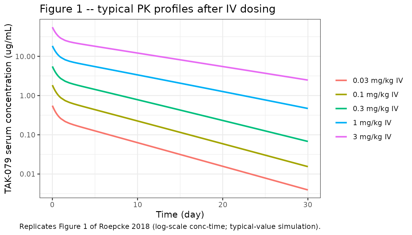
Replicate Figure 1C – IV vs SC (0.3 mg/kg)
The paper’s Figure 1C compares smoothed IV and SC profiles at low
doses. Here we show 0.3 mg/kg IV vs SC in the packaged model – the SC
curve has a slower rise (Ka = 0.399/day) and a substantially smaller
Cmax reflecting the ~70% smaller Vc estimate for SC
(e_route_iv_vc = 0.697).
sim |>
  dplyr::filter(treatment %in% c("0.3 mg/kg IV", "0.3 mg/kg SC")) |>
  ggplot(aes(time, Cc, colour = treatment, linetype = treatment)) +
  geom_line(linewidth = 0.9) +
  scale_y_log10() +
  labs(x = "Time (day)", y = "TAK-079 serum concentration (ug/mL)",
       title = "Figure 1C -- 0.3 mg/kg IV vs SC (typical values)",
       caption = "Replicates Figure 1C of Roepcke 2018.") +
  theme_bw() +
  theme(legend.title = element_blank())
#> Warning in scale_y_log10(): log-10 transformation introduced infinite values.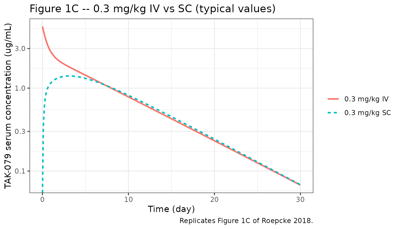
Replicate Figure 4 – lymphocyte depletion profiles
Figure 4 shows the three cell-type depletion profiles (as % of baseline) after IV dosing at 0.1, 0.3, 1 mg/kg. Below we render the typical-value predictions for NK, B, and T cells across the same IV dose levels.
pd_long <- sim |>
  dplyr::filter(ROUTE_IV == 1L, time <= 20) |>
  dplyr::select(treatment, time, nk_pct, b_pct, t_pct) |>
  tidyr::pivot_longer(
    cols       = c(nk_pct, b_pct, t_pct),
    names_to   = "cell",
    values_to  = "pct_baseline"
  ) |>
  dplyr::mutate(
    cell = dplyr::recode(cell,
                         nk_pct = "NK cells",
                         b_pct  = "B cells",
                         t_pct  = "T cells")
  )

ggplot(pd_long, aes(time, pct_baseline, colour = treatment)) +
  geom_line(linewidth = 0.9) +
  geom_hline(yintercept = 50, linetype = "dashed", colour = "grey60") +
  facet_wrap(~ cell) +
  labs(x = "Time (day)", y = "Cell count (% of baseline)",
       title = "Figure 4 -- typical lymphocyte-depletion profiles (IV)",
       caption = "Replicates Figure 4 of Roepcke 2018. 50% dashed line marks a common qualitative cut-off.") +
  theme_bw() +
  theme(legend.title = element_blank())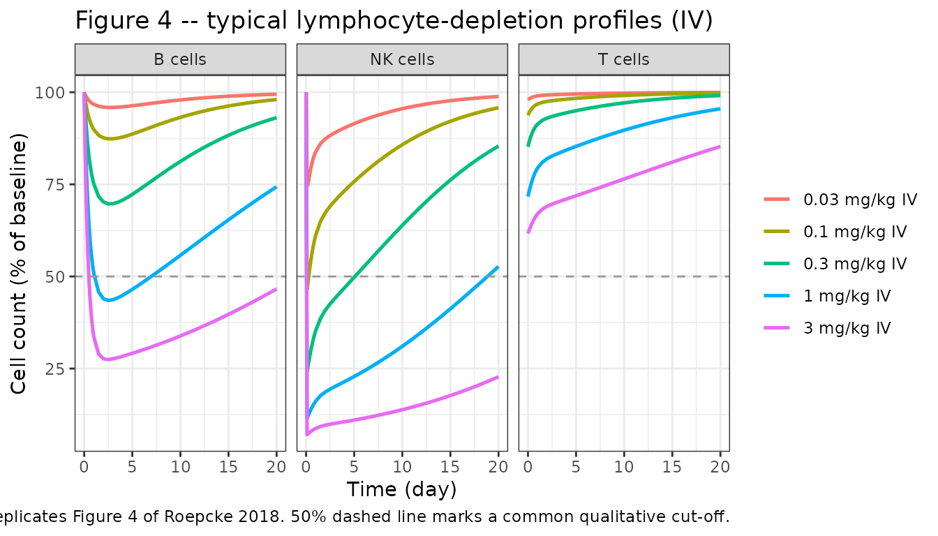
The T-cell curve rises immediately at t = 0 because the T-cell PD
model is a direct response to plasma concentration – with
EMAX = 0.4656, the maximum fractional depletion is roughly
47%, so tcell / BL never falls below ~53% at any
concentration (Roepcke 2018 Section 3.4: “in this case only about half
of the T cells can be depleted by TAK-079”).
PKNCA validation (Cc after single-dose IV / SC)
Compute non-compartmental parameters on the typical-value PK curves for each dose level (single-dose treatments in Roepcke 2018 studies 7 and 8 span the 0.03, 0.1, 0.3, 1 mg/kg IV / SC groups). The paper reports terminal-phase volume of distribution Vz between 64 and 116 mL/kg and clearance between 6.04 and 14.7 mL/kg per day; we compare our simulated central-compartment NCA against those ranges.
# Deduplicate Cc rows -- the event table observes at each time under several
# `cmt` values (Cc / nkcell / bcell / tcell) to trigger every output, so the
# simulation returns four rows per (id, time) that share identical Cc
# values; PKNCA rejects duplicate (id, treatment, time) rows.
sim_nca <- sim |>
  dplyr::filter(!is.na(Cc)) |>
  dplyr::select(id, time, Cc, treatment) |>
  dplyr::group_by(id, treatment, time) |>
  dplyr::slice(1) |>
  dplyr::ungroup()

conc_obj <- PKNCA::PKNCAconc(sim_nca, Cc ~ time | treatment + id)

dose_df <- events |>
  dplyr::filter(evid == 1L) |>
  dplyr::select(id, time, amt, treatment)
dose_obj <- PKNCA::PKNCAdose(dose_df, amt ~ time | treatment + id)

intervals <- data.frame(
  start      = 0,
  end        = Inf,
  cmax       = TRUE,
  tmax       = TRUE,
  aucinf.obs = TRUE,
  half.life  = TRUE
)

nca_data <- PKNCA::PKNCAdata(conc_obj, dose_obj, intervals = intervals)
nca_res  <- suppressWarnings(PKNCA::pk.nca(nca_data))

nca_wide <- as.data.frame(nca_res$result) |>
  dplyr::select(treatment, PPTESTCD, PPORRES) |>
  tidyr::pivot_wider(names_from = PPTESTCD, values_from = PPORRES)

# Derived summary: CL_obs (L/day) = dose / AUCinf,  Vz_obs (mL/kg) = CL / (log(2) / t1/2) / bw_ref * 1000
nca_summary <- nca_wide |>
  dplyr::mutate(
    dose_mg      = as.numeric(sub(" mg/kg .*", "", treatment)) * bw_ref,
    cl_L_per_day = dose_mg / aucinf.obs,
    kel_1perday  = log(2) / half.life,
    vz_L         = cl_L_per_day / kel_1perday,
    cl_mL_per_kg_day = 1000 * cl_L_per_day / bw_ref,
    vz_mL_per_kg     = 1000 * vz_L         / bw_ref
  )

nca_summary |>
  dplyr::select(treatment, cmax, tmax, aucinf.obs, half.life, cl_mL_per_kg_day, vz_mL_per_kg) |>
  dplyr::mutate(dplyr::across(where(is.numeric), ~ round(., 3))) |>
  dplyr::rename(
    "Dose"                    = treatment,
    "Cmax (ug/mL)"            = cmax,
    "Tmax (day)"              = tmax,
    "AUCinf,obs (ug*day/mL)"  = aucinf.obs,
    "t1/2 (day)"              = half.life,
    "CL (mL/kg/day)"          = cl_mL_per_kg_day,
    "Vz (mL/kg)"              = vz_mL_per_kg
  ) |>
  knitr::kable(
    caption = "NCA of typical-value simulated Cc profiles by treatment (dose x route). Compare CL and Vz against Roepcke 2018 Section 3.1: CL 6.04-14.7 mL/kg/day; Vz 64-116 mL/kg (SC data are apparent, not directly comparable)."
)| Dose | Cmax (ug/mL) | Tmax (day) | AUCinf,obs (ug*day/mL) | t1/2 (day) | CL (mL/kg/day) | Vz (mL/kg) |
|---|---|---|---|---|---|---|
| 0.03 mg/kg IV | 0.553 | 0.0 | 1.964 | 4.987 | 15.271 | 109.877 |
| 0.03 mg/kg SC | 0.138 | 3.0 | 1.724 | 5.289 | 17.397 | 132.738 |
| 0.1 mg/kg IV | 1.844 | 0.0 | 6.877 | 5.172 | 14.541 | 108.499 |
| 0.1 mg/kg SC | 0.461 | 3.0 | 5.845 | 5.364 | 17.109 | 132.406 |
| 0.3 mg/kg IV | 5.532 | 0.0 | 23.069 | 5.676 | 13.005 | 106.492 |
| 0.3 mg/kg SC | 1.401 | 3.0 | 18.248 | 5.553 | 16.440 | 131.705 |
| 1 mg/kg IV | 18.440 | 0.0 | 96.020 | 7.063 | 10.415 | 106.114 |
| 1 mg/kg SC | 4.791 | 3.5 | 66.126 | 5.976 | 15.123 | 130.382 |
| 3 mg/kg IV | 55.319 | 0.0 | 352.844 | 8.717 | 8.502 | 106.927 |
Comparison against reported NCA ranges
Roepcke 2018 Section 3.1 (NCA on the single-dose studies) reports:
- Vz (terminal volume of distribution): 64-116 mL/kg
- CL (clearance): 6.04-14.7 mL/kg/day
- Terminal half-life: 4.75-11.2 days
For IV dosing, our typical-value predictions should sit inside these ranges (they reflect the same physiology, aggregated to typical values). SC dosing typically yields lower calculated CL (dose divided by AUCinf, which is dose x F / CL_true) and higher apparent Vz because the SC formulation has ~30% of the IV Vc; the SC apparent-Vz value is not directly comparable to the IV Vz reported in the paper.
Assumptions and deviations
-
Baseline lymphocyte counts. The paper’s models used
individual baselines carried in the dataset (column BL). We use the
paper-reported median baselines from Section 3.3 (NK 685 cells/uL, B
1279 cells/uL, T 3732 cells/uL) as the typical values for
lrbase_nk,lrbase_b,lrbase_t, with BSV etas at the CVs reported in Table 3. -
B-cell transit compartment structure. Section 3.4
reports “five equations” with four transit compartments TR1..TR4
followed by circulating B cells B and the rate constants K_PROL = K_TR =
K_CIRC = 4/MTT, but the five equations themselves are not decoded in the
text extracted from the PDF (Figure text only). We encode the standard
Friberg-style constant-source chain
d/dt(precursor1) = K_TR * (BL - precursor1),d/dt(precursor_{n+1}) = K_TR * (precursor_n - precursor_{n+1}),d/dt(bcell) = K_TR * precursor4 - K_TR * bcell - bcell * EFFwith all rate constants equal to 4/MTT and all initial conditions atrbase_b. This is the parameterisation that (i) reproduces the paper’s steady state at BL when drug is absent, (ii) implements “the drug effect on the depletion rate of circulating B cells” with no feedback on progenitors, and (iii) yields the correct total delay MTT through the chain. Under this encoding TR1 receives a constant source fluxK_PROL * rbase_b, so K_PROL is the paper-reported rate constant with an implicit “reservoir” baseline term equal to the individual baseline; there is no separateProlstate. -
Route-of-administration encoding. The paper models
Vc_SC = Vc * (1 - 0.697)whereSC = 1for SC animals. We use the canonicalROUTE_IVcovariate (1 = IV, 0 = SC) and rewrite asvc = exp(lvc + etalvc) * (1 - e_route_iv_vc * (1 - ROUTE_IV)). IV animals have Vc = 0.141 L; SC animals have Vc = 0.043 L, matching the paper. -
KINT typical value vs BSV. Table 2 reports KINT
typical = 0.1/day as FIXED but the BSV on KINT is 49.3% CV (%SE 36.7).
We encode this as
lkint <- fixed(log(0.1))withetalkint ~ 0.21785estimated – typical value fixed, IIV estimated. -
Residual variance vs SD. Both Table 2 and Table 3
report the “Magnitude” column for residual variability as variances; we
take the square root (
sqrt(...)insideini()) because nlmixr2’s~ prop()and~ add()families expect SDs. -
BSV %CV to variance conversion. The paper reports
BSV as %CV; we use the exact log-normal reverse-transform
omega^2 = log(1 + (CV/100)^2)(so the on-run reported %CV back-reconstructs to Table 2 / Table 3 to within roundoff). This differs from the shorthandomega^2 = (CV/100)^2by <5% up to CV = 50% and matters at CV = 100%+. -
ADA data excluded during model development.
ADA-affected observations (
ADAF = 1, 229 samples) were excluded during the paper’s original fit; this exclusion is not encoded in the packaged model (no ADA covariate). For simulation purposes ADA is not required. SetROUTE_IV = 1for IV cohorts,ROUTE_IV = 0for SC cohorts; no ADA column is used. -
Typical-value simulation vs observed median.
Simulating with
zeroRe()returns the population typical-value prediction, which for the strongly non-linear PD models (especially NK cells, where BSV on bothKINandC50exceeds 100% CV) is systematically shallower than the observed median across animals reported in Section 3.3. This is expected behaviour for log-normal IIV with high CV, not a model-file bug. - T-cell direct-response caveat. Section 3.4 explicitly notes that the direct-response T-cell model under-predicts the initial depletion at the first high dose (e.g., 3 mg/kg group) even though it captures the low-dose and later-time-point behaviour well. We inherit this limitation verbatim; users comparing to Figure 4G-I at high single doses should expect model curves shallower than observed.
-
Human scaling projection is not a fit. The paper’s
Figure 5 simulates human PK / PD by scaling the monkey PK
parameters (
CL_human = CL_monkey * (70 / 2.6)^0.85, etc.) using a straightforward allometric approach for monoclonal antibodies. The packaged model is the monkey fit; users who need the human projection should apply the Supplemental “Scaling of monkey PK parameters” formulas to the loaded model rather than rely on refitted human parameters. - Errata. No published erratum was located for this paper via the text extracted from the PDF; if one exists, please open an issue at https://github.com/nlmixr2/nlmixr2lib.
References
- Roepcke S, Plock N, Yuan J, Fedyk ER, Lahu G, Zhao L, Smithson G. Pharmacokinetics and pharmacodynamics of the cytolytic anti-CD38 human monoclonal antibody TAK-079 in monkey - model assisted preparation for the first in human trial. Pharmacol Res Perspect. 2018;6(3):e00402. doi:10.1002/prp2.402.