N,N-dimethyltryptamine (Eckernas 2022)
Source:vignettes/articles/Eckernas_2022_dimethyltryptamine.Rmd
Eckernas_2022_dimethyltryptamine.RmdModel and source
- Citation: Eckernas E, Timmermann C, Carhart-Harris R, Roshammar D, Ashton M. Population pharmacokinetic/pharmacodynamic modeling of the psychedelic experience induced by N,N-dimethyltryptamine - Implications for dose considerations. Clin Transl Sci. 2022;15(12):2928-2937. doi:10.1111/cts.13410.
- Description: Population PK/PD model of intravenous N,N-dimethyltryptamine (DMT) in healthy adults (Eckernas 2022). Plasma DMT is described by a two-compartment model with first-order elimination from the central compartment; all DMT elimination forms the major metabolite indole-3-acetic acid (IAA, metabolic fraction fixed to 1), whose plasma increment over endogenous baseline follows a one-compartment model with first-order elimination. The subjective intensity of the psychedelic experience (0-10 rating) is driven by the effect-site concentration through a sigmoidal Emax function with zero baseline and Emax fixed to 10, the top of the rating scale. Between-subject variability is on DMT clearance, IAA volume, the effect-site EC50 and the Hill coefficient. Residual error is proportional for DMT and IAA and additive on the logit (0-10) scale for the intensity rating.
- Article: https://doi.org/10.1111/cts.13410 (open access, PMC9747126)
The paper builds one model in three sequential steps: a two-compartment population PK model for plasma DMT, extended with its major metabolite indole-3-acetic acid (IAA), and finally an effect-compartment sigmoidal Emax model for the subjective intensity of the psychedelic experience, fitted with the PK parameters held at their population estimates (“population PK parameters and data” approach). All parameters are in the single Table 1, so the package carries the whole cascade as one model file.
The same authors’ later EEG analysis reuses this PK model with its
parameters fixed; those three models ship as
Eckernas_2023_dimethyltryptamine_alphaPower,
_betaPower and _LZc.
Population
Thirteen healthy volunteers (7 men, 6 women; median age 33 years, range 22-48) took part in a placebo-controlled, fixed-order study at the NIHR Imperial Clinical Research Facility, London. Each received placebo at the first visit and, one week later, a single intravenous bolus of DMT fumarate: 7 mg (n = 3), 14 mg (n = 4), 18 mg (n = 1) or 20 mg (n = 5). Nine plasma samples per subject were taken up to 60 min after dosing, and the subject rated the intensity of the experience on a 0-10 scale (0 = no effect, 10 = the most intense experience imaginable) every minute for the first 20 min. The analysis used 93 DMT and 87 IAA concentrations and 273 intensity ratings (Results, first paragraph). Placebo-visit data showed no measurable DMT and no subjective effect and were not modelled. The paper does not tabulate body weight or race.
The same information is available programmatically via
readModelDb("Eckernas_2022_dimethyltryptamine")()$population.
Source trace
Every ini() value carries an in-file comment naming its
source. The table collects them.
| Equation / parameter | Value | Source location |
|---|---|---|
lcl (DMT CL) |
26.0 L/min | Table 1 |
lvc (DMT Vc) |
221 L | Table 1 |
lq (DMT Q) |
2.99 L/min | Table 1 |
lvp (DMT Vp) |
59.0 L | Table 1 |
fm (fraction of DMT elimination forming IAA) |
1 (fixed) | Methods, Pharmacokinetic model development |
lcl_iaa (CL(m)) |
0.093 L/min | Table 1 |
lvc_iaa (V(m)) |
9.55 L | Table 1 |
emax |
10 (fixed) | Table 1; Results, PK/PD model |
lec50 (EC50,e) |
94.7 nM | Table 1 |
lke0 |
1.38 1/min | Table 1 |
lhill (gamma) |
2.87 | Table 1 |
etalcl |
0.473^2 = 0.2237 | Table 1, BSV CL 47.3 %CV |
etalvc_iaa |
0.290^2 = 0.0841 | Table 1, BSV V(m) 29.0 %CV |
etalec50 |
0.386^2 = 0.1490 | Table 1, BSV EC50,e 38.6 %CV |
etalhill |
0.773^2 = 0.5975 | Table 1, BSV gamma 77.3 %CV |
propSd (DMT) |
0.500 | Table 1, residual error DMT 50.0 %CV |
propSd_iaa |
0.190 | Table 1, residual error IAA 19.0 %CV |
addSd_psychedelicintensity |
0.82 (logit scale) | Table 1; Equation 1 |
d/dt(central), d/dt(peripheral1)
|
two-compartment, first-order elimination | Methods; Results, Population PK model |
d/dt(central_iaa) = fm * kel * central - kel_iaa * central_iaa |
n/a | Methods: IAA formation rate equals the DMT elimination rate |
d/dt(effect) = ke0 * (Cc - effect) |
n/a | Methods, effect-compartment equation |
psychedelicintensity = emax * Ce^gamma / (EC50^gamma + Ce^gamma) |
E0 = 0 | Methods, Emax equation; Results: all subjects had a baseline of zero |
psychedelicintensity ~ logitNorm(sd, 0, 10) |
n/a | Equation 1:
y = 10 * exp(ln(lambda/(10 - lambda)) + eps) / (1 + exp(...))
|
Dose units
The model runs in molar units: doses are nmol of DMT base and
concentrations are nmol/L (= nM), the unit of EC50,e. The paper states
doses as mg of DMT fumarate and that they “were converted and expressed
as nanomoles of DMT base”, without printing the factor. The vignette
uses the 1:1 salt stoichiometry,
DMT (C12H16N2, 188.27 g/mol) + fumaric acid (C4H4O4, 116.07 g/mol),
giving 304.34 g/mol, or 3286 nmol DMT base per mg of salt.
mw_dmt      <- 188.27
mw_fumarate <- 116.07
nmolPerMg   <- 1e6 / (mw_dmt + mw_fumarate)
doseMg      <- c(1, 4, 7, 14, 20)  # Figure 4 simulation doses (mg DMT fumarate)
tibble(
  `Dose (mg DMT fumarate)` = doseMg,
  `Dose (nmol DMT base)`   = round(doseMg * nmolPerMg),
  `C0 = Dose / Vc (nM)`    = round(doseMg * nmolPerMg / 221, 1)
) |>
knitr::kable(caption = "Molar dose conversion used throughout this vignette.")| Dose (mg DMT fumarate) | Dose (nmol DMT base) | C0 = Dose / Vc (nM) |
|---|---|---|
| 1 | 3286 | 14.9 |
| 4 | 13143 | 59.5 |
| 7 | 23001 | 104.1 |
| 14 | 46001 | 208.2 |
| 20 | 65716 | 297.4 |
Virtual cohort
The paper’s Figure 4 simulated 100 subjects at each of five IV bolus doses. The vignette uses 200 subjects per dose, the most it permits, so that the dose-response statistics checked below sit well clear of Monte-Carlo noise. No covariates enter the model.
# rxSetSeed() fixes rxode2's draw for a given solver thread count only, so the
# assertions below are written to hold for any cohort the model can produce.
rxode2::rxSetSeed(2022)
set.seed(2022)

nPerDose <- 200L
obsGrid  <- seq(0, 60, by = 0.25)

make_cohort <- function(n, mg, id_offset) {
  ids <- id_offset + seq_len(n)
  dose <- tibble(id = ids, time = 0, amt = mg * nmolPerMg, evid = 1L,
                 cmt = "central", dvid = NA_integer_)
  obs  <- tidyr::expand_grid(id = ids, time = obsGrid) |>
    mutate(amt = 0, evid = 0L, cmt = "central", dvid = 1L)
  bind_rows(dose, obs) |>
    mutate(dose_mg = mg) |>
    arrange(id, time, desc(evid))
}

events <- bind_rows(lapply(seq_along(doseMg), function(i) {
  make_cohort(nPerDose, doseMg[i], id_offset = (i - 1L) * nPerDose)
}))
stopifnot(!anyDuplicated(unique(events[, c("id", "time", "evid")])))
Simulation
Observation rows are placed on the central state with
dvid = 1; rxode2 returns every model variable
(Cc, Cc_iaa,
psychedelicintensity) on each row. Residual error is added
afterwards in R, following the paper’s definitions, so each endpoint
gets its own draw.
mod <- readModelDb("Eckernas_2022_dimethyltryptamine")
sim <- rxode2::rxSolve(mod, events = events, keep = "dose_mg",
                       returnType = "data.frame") |>
  mutate(
    dose = factor(paste(dose_mg, "mg"), levels = paste(doseMg, "mg")),
    # Proportional residual error on DMT and IAA (Table 1).
    Cc_obs     = Cc * (1 + 0.500 * rnorm(n())),
    Cc_iaa_obs = Cc_iaa * (1 + 0.190 * rnorm(n())),
    # Equation 1: additive error on the logit scale bounded by 0 and 10.
    rating_obs = 10 * plogis(qlogis(psychedelicintensity / 10) + 0.82 * rnorm(n()))
  )
#> ℹ parameter labels from comments will be replaced by 'label()'
stopifnot(!anyNA(sim$Cc), !anyNA(sim$Cc_iaa), !anyNA(sim$psychedelicintensity))
Replicate published figures
Figure 1 – DMT and IAA concentrations by dose
Observed medians in Figure 1b-c are drawn as approximate points read off the published figure by the maintainers. The study’s 18 mg and 20 mg subjects were pooled in that figure; the simulation shows 20 mg.
fig1_obs <- tribble(
  ~analyte, ~dose,   ~time, ~conc,
  "IAA",    "7 mg",   5,    1200,
  "IAA",    "7 mg",  26,    1900,
  "IAA",    "7 mg",  44,    1550,
  "IAA",    "7 mg",  60,    1550,
  "IAA",    "14 mg",  5,    2000,
  "IAA",    "14 mg", 20,    3100,
  "IAA",    "14 mg", 40,    3200,
  "IAA",    "14 mg", 60,    3050,
  "IAA",    "20 mg",  3,    2900,
  "IAA",    "20 mg", 20,    4700,
  "IAA",    "20 mg", 38,    4750,
  "IAA",    "20 mg", 60,    4300,
  "DMT",    "7 mg",   2,      45,
  "DMT",    "7 mg",   5,      30,
  "DMT",    "14 mg",  3,     105,
  "DMT",    "14 mg",  5,     100,
  "DMT",    "20 mg",  2,     135,
  "DMT",    "20 mg",  5,     130,
  "DMT",    "20 mg", 20,      18
) |>
  mutate(dose = factor(dose, levels = paste(doseMg, "mg")))

sim |>
  filter(dose_mg %in% c(7, 14, 20), time > 0) |>
  select(dose, time, DMT = Cc_obs, IAA = Cc_iaa_obs) |>
  pivot_longer(c(DMT, IAA), names_to = "analyte", values_to = "conc") |>
  group_by(analyte, dose, time) |>
  summarise(Q05 = quantile(conc, 0.05), Q50 = median(conc),
            Q95 = quantile(conc, 0.95), .groups = "drop") |>
  ggplot(aes(time, Q50)) +
  geom_ribbon(aes(ymin = Q05, ymax = Q95), alpha = 0.25, fill = "steelblue") +
  geom_line(colour = "steelblue4") +
  geom_point(data = fig1_obs, aes(time, conc), colour = "black") +
  facet_grid(analyte ~ dose, scales = "free_y") +
  labs(x = "Time (min)", y = "Concentration (nM)",
       title = "Figure 1 -- simulated DMT and IAA (median, 5th-95th percentile)",
       caption = "Replicates Figure 1b-c of Eckernas 2022. Points: approximate observed medians read from the figure.")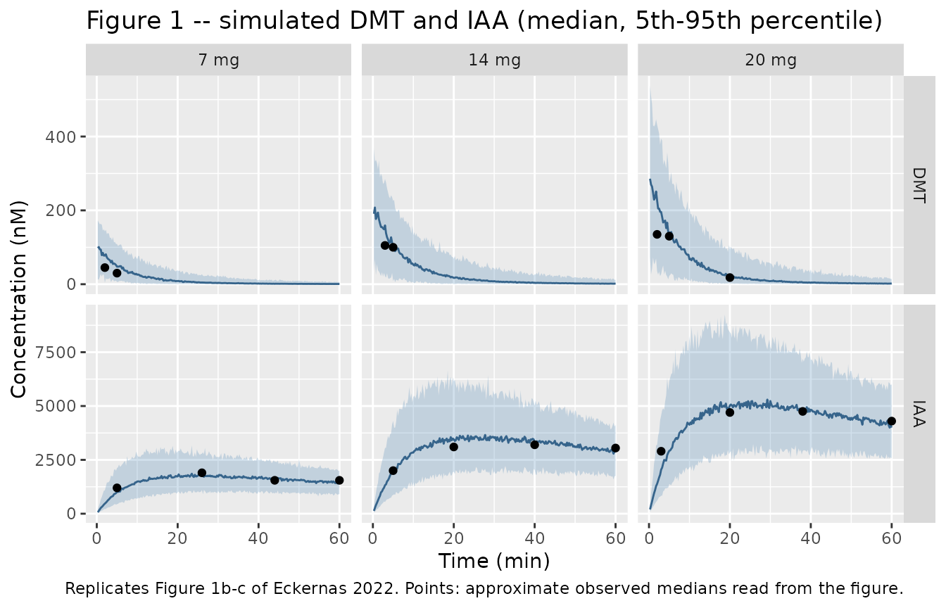
The simulated IAA medians follow the observed medians at all three
dose levels. Once DMT has been eliminated, the IAA level is set mainly
by the molar dose and V(m), so this agreement supports the
dose conversion. The early DMT medians lie somewhat above the observed
values at 2-5 min. Those observed values come from three to six subjects
per panel, and the 18/20 mg panel includes the one 18 mg subject.
Figure 2 – intensity rating versus time
fig2_obs <- tribble(
  ~dose,   ~time, ~rating,
  "7 mg",    2.5,  4.5,
  "7 mg",    7,    5,
  "7 mg",   15.5,  2,
  "14 mg",   2.5,  7,
  "14 mg",   7,    4,
  "14 mg",  15.5,  1,
  "20 mg",   2.5,  9.5,
  "20 mg",   7,    8,
  "20 mg",  15.5,  1
) |>
  mutate(dose = factor(dose, levels = paste(doseMg, "mg")))

sim |>
  filter(dose_mg %in% c(7, 14, 20), time <= 20) |>
  group_by(dose, time) |>
  summarise(Q05 = quantile(rating_obs, 0.05), Q50 = median(rating_obs),
            Q95 = quantile(rating_obs, 0.95), .groups = "drop") |>
  ggplot(aes(time, Q50)) +
  geom_ribbon(aes(ymin = Q05, ymax = Q95), alpha = 0.25, fill = "firebrick") +
  geom_line(colour = "firebrick4") +
  geom_point(data = fig2_obs, aes(time, rating), colour = "black") +
  facet_wrap(~dose) +
  coord_cartesian(ylim = c(0, 10)) +
  labs(x = "Time (min)", y = "Subjective intensity rating",
       title = "Figure 2 -- simulated intensity rating (median, 5th-95th percentile)",
       caption = "Replicates Figure 2b of Eckernas 2022. Points: approximate observed medians read from the figure.")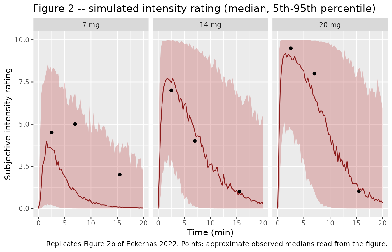
The 14 mg and 20 mg simulated medians track the observed medians. At 7 mg the observed medians come from only three subjects and lie above the simulated median after the peak; they fall inside the simulated 5th-95th percentile band, as they do inside the paper’s own prediction interval for that panel.
Figure 4 – maximum achieved intensity by dose
Figure 4 shows the distribution of each simulated subject’s maximum rating over the 20-min rating window. The vignette takes the maximum of the individual prediction (no residual error), which reproduces the published boxes; the paper does not say whether residual error was included.
maxRating <- sim |>
  filter(time <= 20) |>
  group_by(dose, dose_mg, id) |>
  summarise(max_rating = max(psychedelicintensity), .groups = "drop")

# Figure 4 whiskers span the 5th-95th percentiles.
maxRating |>
  group_by(dose) |>
  summarise(
    ymin   = quantile(max_rating, 0.05),
    lower  = quantile(max_rating, 0.25),
    middle = median(max_rating),
    upper  = quantile(max_rating, 0.75),
    ymax   = quantile(max_rating, 0.95),
    .groups = "drop"
  ) |>
  ggplot(aes(dose, ymin = ymin, lower = lower, middle = middle,
             upper = upper, ymax = ymax)) +
  geom_boxplot(stat = "identity") +
  labs(x = "Dose (mg DMT fumarate)", y = "Maximum subjective intensity rating",
       title = "Figure 4 -- maximum achieved intensity",
       caption = "Replicates Figure 4 of Eckernas 2022.")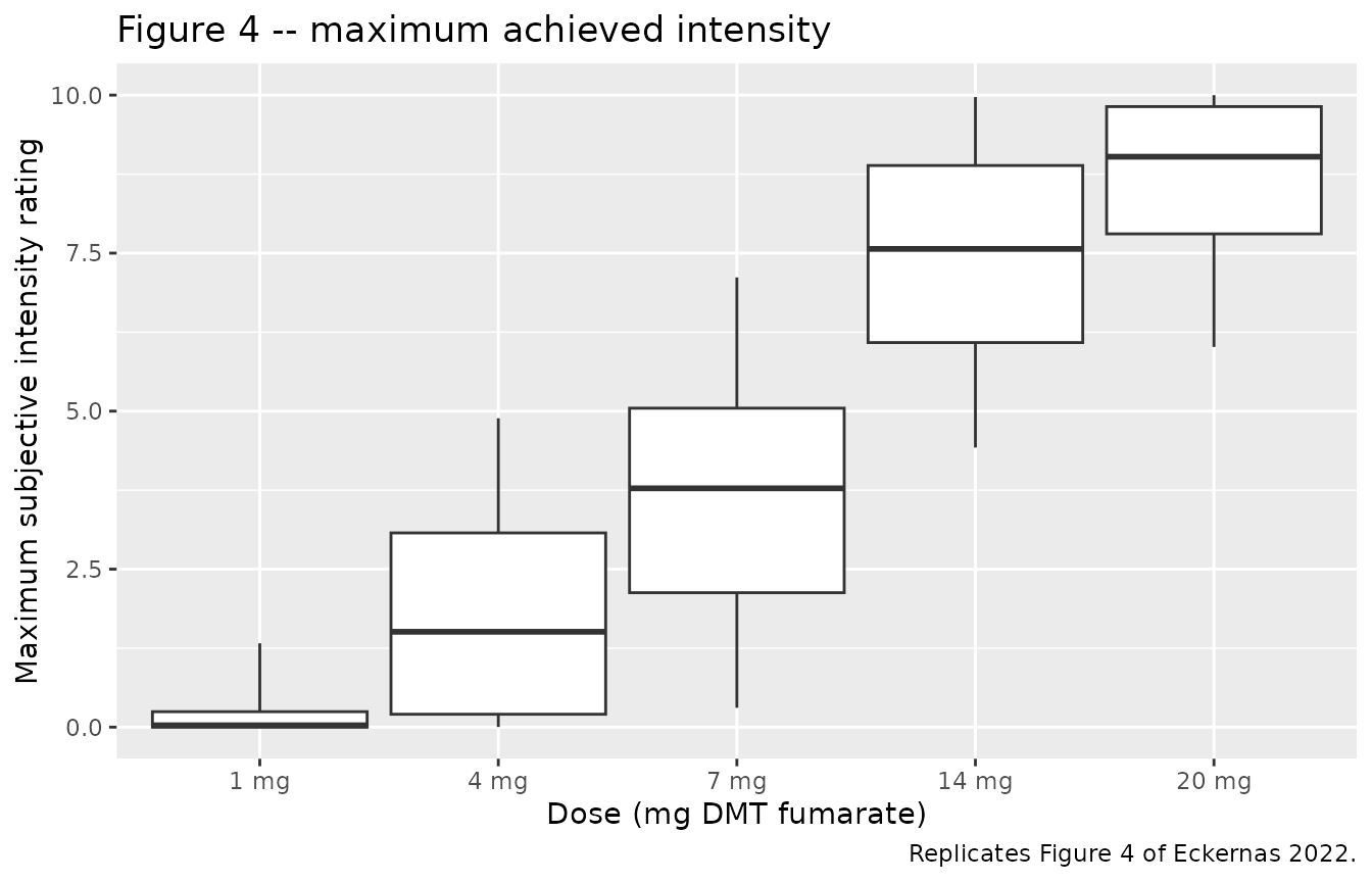
# Medians of the Figure 4 boxes (read from the figure) and the Results text:
# "A median maximum effect of 0, 2, 4, 8, and 9 ... The proportion of the
# population achieving a maximum rating above five increased from zero at the
# lowest dose to 4, 42, 92, and 100%".
published4 <- tibble(
  dose_mg        = doseMg,
  median_figure  = c(0, 1.35, 3.95, 7.95, 9.2),
  median_text    = c(0, 2, 4, 8, 9),
  pct_above5     = c(0, 4, 42, 92, 100)
)
fig4 <- maxRating |>
  group_by(dose_mg) |>
  summarise(sim_median = median(max_rating),
            sim_pct_above5 = 100 * mean(max_rating > 5), .groups = "drop") |>
  left_join(published4, by = "dose_mg")

fig4 |>
  mutate(across(where(is.double), ~ round(.x, 2))) |>
  rename(
    "Dose (mg)"                  = dose_mg,
    "Simulated median max"       = sim_median,
    "Simulated % max > 5"        = sim_pct_above5,
    "Figure 4 median"            = median_figure,
    "Text median"                = median_text,
    "Published % max > 5"        = pct_above5
  ) |>
knitr::kable(caption = "Maximum rating by dose: simulated versus Eckernas 2022.")| Dose (mg) | Simulated median max | Simulated % max > 5 | Figure 4 median | Text median | Published % max > 5 |
|---|---|---|---|---|---|
| 1 | 0.03 | 0.0 | 0.00 | 0 | 0 |
| 4 | 1.51 | 4.5 | 1.35 | 2 | 4 |
| 7 | 3.78 | 27.5 | 3.95 | 4 | 42 |
| 14 | 7.57 | 91.5 | 7.95 | 8 | 92 |
| 20 | 9.03 | 98.0 | 9.20 | 9 | 100 |
# A 3000-subject-per-dose run of this model gives medians 0.02 / 1.35 / 4.12 /
# 7.90 / 9.10 and percentages above 5 of 0 / 3.0 / 34.8 / 91.1 / 98.7. With 200
# subjects per dose the standard error of a median is about 0.2 rating units and
# of a percentage at most 3.5 points, so the bounds below are ~4 standard
# errors wide. The 7 mg percentage sits furthest from the paper (model 35%
# versus 42%); one 200-subject draw realised 27.5%, inside the bound. A two-fold
# error in EC50, a dose or a unit moves the 7 mg and 14 mg medians by several
# units and fails them.
stopifnot(
  all(abs(fig4$sim_median - fig4$median_figure) < 0.8),
  all(abs(fig4$sim_pct_above5 - fig4$pct_above5) < 20)
)
The simulated medians agree with the Figure 4 boxes. The Results text rounds the 4 mg median to 2, whereas the figure box and the model sit at about 1.4. The model’s share of 7 mg subjects above a rating of 5 is about 35%, against 42% in the text; the paper’s own 100-subject simulation carries a standard error of about 5 points on that figure.
PKNCA validation
The paper reports no NCA table. The check below runs PKNCA on a
typical-value solve and compares against quantities the model implies in
closed form: DMT AUC0-inf = Dose / CL, IAA
AUC0-inf = fm * Dose / CL(m) (independent of the DMT
parameters because every mole of DMT becomes IAA), the DMT terminal
half-life from the two-compartment eigenvalue, and the IAA half-life
ln(2) * V(m) / CL(m), which is the slowest rate in the
system.
ncaDoseMg <- c(7, 14, 20)
ncaGrid <- sort(unique(c(seq(0, 10, by = 0.1), seq(10, 720, by = 2))))
ncaEvents <- bind_rows(lapply(seq_along(ncaDoseMg), function(i) {
  bind_rows(
    tibble(id = i, time = 0, amt = ncaDoseMg[i] * nmolPerMg, evid = 1L,
           cmt = "central", dvid = NA_integer_),
    tibble(id = i, time = ncaGrid, amt = 0, evid = 0L, cmt = "central", dvid = 1L)
  ) |>
    mutate(treatment = paste(ncaDoseMg[i], "mg"))
}))

# Typical values: omega = NA and sigma = NA drop all random effects.
typ <- rxode2::rxSolve(mod, events = ncaEvents, omega = NA, sigma = NA,
                       keep = "treatment", rtol = 1e-10, atol = 1e-12,
                       returnType = "data.frame")

concLong <- bind_rows(
  # DMT falls ~13 terminal half-lives by 240 min; later points are solver noise.
  typ |> filter(time <= 240) |> transmute(id, time, treatment, analyte = "DMT", Cc),
  typ |> transmute(id, time, treatment, analyte = "IAA", Cc = Cc_iaa)
) |>
  filter(!is.na(Cc))
stopifnot(all(concLong$Cc >= -1e-6 * max(concLong$Cc)))
concLong$Cc <- pmax(concLong$Cc, 0)

conc_obj <- PKNCA::PKNCAconc(concLong, Cc ~ time | analyte + treatment + id)
dose_obj <- PKNCA::PKNCAdose(
  ncaEvents |> filter(evid == 1) |> select(id, time, amt, treatment),
  amt ~ time | treatment + id
)
intervals <- data.frame(start = 0, end = Inf, cmax = TRUE, tmax = TRUE,
                        aucinf.obs = TRUE, half.life = TRUE)
nca_res <- PKNCA::pk.nca(PKNCA::PKNCAdata(conc_obj, dose_obj, intervals = intervals))
th <- list(cl = 26.0, vc = 221, q = 2.99, vp = 59.0, cl_iaa = 0.093, vc_iaa = 9.55)
kel <- th$cl / th$vc
k12 <- th$q / th$vc
k21 <- th$q / th$vp
beta <- ((kel + k12 + k21) - sqrt((kel + k12 + k21)^2 - 4 * kel * k21)) / 2

reference <- tidyr::expand_grid(analyte = c("DMT", "IAA"), dmg = ncaDoseMg) |>
  mutate(
    treatment  = paste(dmg, "mg"),
    doseNmol   = dmg * nmolPerMg,
    aucinf.obs = ifelse(analyte == "DMT", doseNmol / th$cl, doseNmol / th$cl_iaa),
    half.life  = ifelse(analyte == "DMT", log(2) / beta, log(2) * th$vc_iaa / th$cl_iaa),
    cmax       = ifelse(analyte == "DMT", doseNmol / th$vc, NA_real_)
  ) |>
  select(analyte, treatment, cmax, aucinf.obs, half.life)

cmp <- nlmixr2lib::ncaComparisonTable(
  simulated = nca_res,
  reference = reference,
  by        = c("analyte", "treatment"),
  params    = c("cmax", "aucinf.obs", "half.life"),
  units     = c(cmax = "nM", aucinf.obs = "nM*min", half.life = "min"),
  tolerance_pct = 5
)
knitr::kable(cmp, caption = "PKNCA on the typical-value solve versus the model's closed-form values. * differs by >5%.")| NCA parameter | analyte | treatment | Reference | Simulated | % diff |
|---|---|---|---|---|---|
| Cmax (nM) | DMT | 7 mg | 104 | 104 | +0.0% |
| Cmax (nM) | DMT | 14 mg | 208 | 208 | +0.0% |
| Cmax (nM) | DMT | 20 mg | 297 | 297 | +0.0% |
| Cmax (nM) | IAA | 7 mg | — | 1820 | — |
| Cmax (nM) | IAA | 14 mg | — | 3650 | — |
| Cmax (nM) | IAA | 20 mg | — | 5210 | — |
| AUC0-∞ (obs) (nM*min) | DMT | 7 mg | 885 | 885 | +0.0% |
| AUC0-∞ (obs) (nM*min) | DMT | 14 mg | 1770 | 1770 | +0.0% |
| AUC0-∞ (obs) (nM*min) | DMT | 20 mg | 2530 | 2530 | +0.0% |
| AUC0-∞ (obs) (nM*min) | IAA | 7 mg | 247000 | 247000 | -0.0% |
| AUC0-∞ (obs) (nM*min) | IAA | 14 mg | 495000 | 495000 | -0.0% |
| AUC0-∞ (obs) (nM*min) | IAA | 20 mg | 707000 | 707000 | -0.0% |
| t½ (min) | DMT | 7 mg | 16.2 | 16.1 | -0.6% |
| t½ (min) | DMT | 14 mg | 16.2 | 16.1 | -0.6% |
| t½ (min) | DMT | 20 mg | 16.2 | 16.1 | -0.6% |
| t½ (min) | IAA | 7 mg | 71.2 | 71.5 | +0.4% |
| t½ (min) | IAA | 14 mg | 71.2 | 71.5 | +0.4% |
| t½ (min) | IAA | 20 mg | 71.2 | 71.5 | +0.4% |
# Deterministic solve against its own closed form: the residual is numerical
# (trapezoid and terminal-slope fit), measured below 1%.
pp <- as.data.frame(nca_res) |>
  filter(PPTESTCD %in% c("aucinf.obs", "half.life")) |>
  left_join(reference |> pivot_longer(c(aucinf.obs, half.life),
                                      names_to = "PPTESTCD", values_to = "ref") |>
              select(analyte, treatment, PPTESTCD, ref),
            by = c("analyte", "treatment", "PPTESTCD"))
stopifnot(nrow(pp) == 12L, all(abs(pp$PPORRES / pp$ref - 1) < 0.02))
The DMT Cmax row is the time-zero concentration of the
bolus, Dose / Vc. IAA has no closed-form Cmax
and is omitted from that row.
Assumptions and deviations
-
Molar dose conversion. The paper converts DMT
fumarate doses to nmol of DMT base without printing the factor. The
vignette uses 1:1 salt stoichiometry (304.34 g/mol, 3286 nmol/mg). The
sibling
Eckernas_2023_dimethyltryptamine_EEGarticle infers about 3150 nmol/mg from a figure axis, 4% lower. The Figure 4 medians reproduced here, which depend on the conversion through EC50,e, support the stoichiometric value. -
Variance scale of the BSV terms. Table 1 reports
BSV as %CV without stating the conversion. The variances are
(CV/100)^2, because the same authors’ 2023 analysis carries BSV on CL forward as$OMEGA 0.224 FIX, which is0.473^2rather thanlog(1 + 0.473^2) = 0.201. The other three BSV terms were converted the same way. -
PK parameters are the paper’s estimates. In the
final PK/PD step the population PK parameters were held at their PK-step
estimates. The library model presents all of Table 1 as one model, so
the PK values are the estimated values and are not wrapped in
fixed();Emax = 10and the metabolic fraction of 1, which the paper held constant, arefixed(). -
IAA baseline. IAA was assayed as the change from
the endogenous baseline, so
Cc_iaais the DMT-derived increment and starts at zero. - Correlation between EC50,e and gamma. The paper estimated a 93% correlation between those two random effects but dropped it from the final model for ill-conditioning. The model follows the final, uncorrelated form.
- Rating at zero concentration. With a zero baseline the prediction is 0 before dosing, where the logit transform in Equation 1 is undefined. The paper notes that the transform only approaches the scale limits asymptotically. In this vignette the residual draw at a zero prediction returns 0.
- Figure 4 maximum. The maximum rating is taken from the individual prediction without residual error, over a 0.25-min grid from 0 to 20 min.
- Observed medians overlaid on Figures 1 and 2 are approximate values read from the published figures by the maintainers and are not used in any assertion.
- No erratum for this article was found on the publisher page or in Europe PMC as of 2026-10-10.