Ciclosporin (Fanta 2007)
Source:vignettes/articles/Fanta_2007_ciclosporin.Rmd
Fanta_2007_ciclosporin.RmdModel and source
- Citation: Fanta S, Jonsson S, Backman JT, Karlsson MO, Hoppu K. Developmental pharmacokinetics of ciclosporin – a population pharmacokinetic study in paediatric renal transplant candidates. Br J Clin Pharmacol. 2007;64(6):772-784.
- Article: https://doi.org/10.1111/j.1365-2125.2007.03003.x
- Description: Three-compartment population PK model with first-order absorption for ciclosporin in paediatric renal transplant candidates.
Population
The dataset comprised 162 of 166 paediatric renal transplant candidates studied at the Hospital for Children and Adolescents, University of Helsinki between 1988 and 2005 (Fanta 2007 Table 1). All patients had renal disease (congenital nephrosis of the Finnish type, urethral valve, polycystic renal disease, nephronophtisis, or other diagnoses) and were on continuous ambulatory or continuous cycling peritoneal dialysis prior to renal transplantation. The median age was 3.8 years (range 0.36-17.5 years), mean body weight was 22.2 +/- 15.7 kg (range 6.9-64 kg), and 107 of 162 patients (66%) were male. One patient was of East African descent and the remaining 161 were Finnish Whites.
Ciclosporin was administered as a 3 mg/kg 4-hour intravenous infusion (Sandimmun) and, on a separate occasion at least 24 h later, as a 10 mg/kg single oral dose of the microemulsion formulation (Sandimmun Neoral). Of the 162 patients, all contributed IV data and 89 contributed oral microemulsion data; the 73 patients who received the conventional (non-microemulsion) oral formulation were excluded from the population model because that formulation is no longer used. Concentrations were measured in 1 mL EDTA whole blood by a specific monoclonal radioimmunoassay (Sandoz Sandimmune Kit until May 1994, Incstar / DiaSorin CycloTrac thereafter; LOD ~5 ug/L, within- and between-run CV < 7% for concentrations > 30 ug/L). 2437 concentration records contributed to the popPK analysis (Fanta 2007 Results “Structural and stochastic models” paragraph 1).
The same baseline summary is available programmatically via
readModelDb("Fanta_2007_ciclosporin")$population.
Source trace
The per-parameter origin is recorded as an in-file comment next to
each ini() entry of
inst/modeldb/specificDrugs/Fanta_2007_ciclosporin.R. The
table below collects them in one place for review.
| Equation / parameter | Value | Source location |
|---|---|---|
lka (ka, 1/h) |
log(0.68) | Fanta 2007 Table 2 (“Absorption rate constant Ka”) |
lcl (apparent CL, oral arm, L/h) |
log(0.77 * 6.1) | Fanta 2007 Table 2 (IV CL = 6.1) and Results “Structural and stochastic models” paragraph 4 (oral CL is 23% lower than IV CL) |
lvc (V2, L) |
log(5.3) | Fanta 2007 Table 2 |
lq (Q3, L/h) |
log(1.5) | Fanta 2007 Table 2 |
lvp (V3, L) |
log(19.6) | Fanta 2007 Table 2 |
lq2 (Q4, L/h) |
log(3.0) | Fanta 2007 Table 2 |
lvp2 (V4, L) |
log(4.4) | Fanta 2007 Table 2 |
lfdepot (F, fraction) |
log(0.36) | Fanta 2007 Table 2 (“Oral bioavailability F”) |
e_wt_cl (allometric on CL/Q3/Q4) |
fixed(0.75) | Fanta 2007 Results “Covariate model” paragraph 1 (fixed at theoretical 3/4) |
e_wt_vc (allometric on V2/V3/V4) |
fixed(1.0) | Fanta 2007 Results “Covariate model” paragraph 1 (fixed at theoretical 1) |
e_tchol_cl (1/(mmol/L)) |
-0.0542 | Fanta 2007 Table 2 footnote / Figure 5 caption |
e_hct_cl (1/%) |
-0.00732 | Fanta 2007 Table 2 footnote / Figure 5 caption |
e_creat_cl (1/(umol/L)) |
0.000214 | Fanta 2007 Table 2 footnote / Figure 5 caption |
e_route_iv_cl (log-shift IV vs oral CL) |
log(1/0.77) ~= 0.2614 | Fanta 2007 Results “Structural and stochastic models” paragraph 4 |
Shared eta block for etalvc, etalq2,
etalvp2
|
omega^2 = log(CV^2 + 1) with CVs 12% / 39% / 25%; off-diagonals under full positive correlation | Fanta 2007 Table 2 (IIV V2, Q4, V4) + Results paragraph 1 (“V2, V4, Q4 shared the same eta”) |
etalcl |
log(1 + 0.17^2) = 0.0285 | Fanta 2007 Table 2 (IIV CL CV = 17%) |
etalq |
log(1 + 0.31^2) = 0.0917 | Fanta 2007 Table 2 (IIV Q3 CV = 31%) |
etalvp |
log(1 + 0.42^2) = 0.1625 | Fanta 2007 Table 2 (IIV V3 CV = 42%) |
etalka |
log(1 + 0.33^2) = 0.1034 | Fanta 2007 Table 2 (IIV Ka CV = 33%) |
etalfdepot |
log(1 + 0.11^2) = 0.0120 | Fanta 2007 Table 2 (IIV F CV = 11%) |
propSdPo (oral arm proportional) |
0.20 | Fanta 2007 Table 2 |
propSdIv (IV arm proportional) |
0.089 | Fanta 2007 Table 2 |
addSdIv (IV arm additive, ug/L) |
1.5 | Fanta 2007 Table 2 |
| Three-compartment ODE system with first-order absorption from depot | n/a | Fanta 2007 Results “Structural and stochastic models” paragraph 1 (3-compartment model with first-order absorption without lag-time) |
Allometric scaling formula (WT / 13)^A with A = 3/4 on
CL/Q and A = 1 on V |
n/a | Fanta 2007 Table 2 footnote |
Shared linear-deviation covariate factor
(1 + e * (X - ref)) applied to every CL and every V
parameter |
n/a | Fanta 2007 Table 2 footnote and Results “Covariate model” paragraph 2 |
Virtual cohort
The original observed data are not publicly available. The figures below use a virtual paediatric cohort whose body-weight and reference-covariate distributions approximate the Fanta 2007 Table 1 cohort. Each subject contributes one IV occasion (3 mg/kg, 4-hour infusion) and one oral occasion (10 mg/kg, microemulsion), matching the paper’s two-arm pretransplantation study design.
set.seed(20070719)

n_subj <- 60L

# Reference covariates per Fanta 2007 Table 2 footnote.
ref_wt    <- 13
ref_tchol <- 5.4
ref_hct   <- 31
ref_creat <- 524

# Build per-subject demographics drawn approximately from Table 1 ranges.
# (BW range 6.9-64 kg; we sample log-uniformly so the cohort spans the full
# paediatric range without over-weighting heavy adolescents.)
subjects <- tibble(
  id     = seq_len(n_subj),
  WT     = round(exp(seq(log(6.9), log(64), length.out = n_subj)), 1),
  TCHOL  = round(rnorm(n_subj, mean = ref_tchol, sd = 1.6), 2),
  HCT    = round(rnorm(n_subj, mean = ref_hct,   sd = 7),    1),
  CREAT  = round(rnorm(n_subj, mean = ref_creat, sd = 252),  1)
) |>
  mutate(
    TCHOL = pmax(3.1, pmin(9.8, TCHOL)),
    HCT   = pmax(15,  pmin(48,  HCT)),
    CREAT = pmax(165, pmin(1669, CREAT))
  )

make_cohort <- function(subj, route_label, id_offset = 0L) {
  # Per-subject dose amount based on the paper's mg/kg regimen.
  doses_iv <- subj |>
    mutate(amt = 3  * WT, time = 0, evid = 1, cmt = "central",
           dur = 4, ROUTE_IV = 1L, occ = "IV")
  doses_po <- subj |>
    mutate(amt = 10 * WT, time = 0, evid = 1, cmt = "depot",
           dur = NA_real_, ROUTE_IV = 0L, occ = "PO")

  if (route_label == "IV") doses <- doses_iv else doses <- doses_po

  obs_grid <- c(0, 1, 2, 3, 4, 6, 9, 12, 16, 24)
  obs <- subj |>
    tidyr::crossing(time = obs_grid) |>
    mutate(amt = NA_real_, evid = 0, cmt = "central",
           dur = NA_real_,
           ROUTE_IV = if (route_label == "IV") 1L else 0L,
           occ = route_label)

  dplyr::bind_rows(doses, obs) |>
    mutate(id = id + id_offset) |>
    arrange(id, time, desc(evid))
}

events <- dplyr::bind_rows(
  make_cohort(subjects, "IV", id_offset = 0L),
  make_cohort(subjects, "PO", id_offset = n_subj)
)

stopifnot(!anyDuplicated(unique(events[, c("id", "time", "evid")])))
Simulation
mod <- readModelDb("Fanta_2007_ciclosporin")
sim <- rxode2::rxSolve(mod, events = events,
                       keep = c("occ", "WT")) |>
  as.data.frame()
#> ℹ parameter labels from comments will be replaced by 'label()'
For deterministic replication (typical-value Figure 2 reproduction), zero out the random effects.
mod_typ <- rxode2::zeroRe(mod)
#> ℹ parameter labels from comments will be replaced by 'label()'
#> Warning: No sigma parameters in the model
sim_typ <- rxode2::rxSolve(mod_typ, events = events,
                           keep = c("occ", "WT")) |>
  as.data.frame()
#> ℹ omega/sigma items treated as zero: 'etalvc', 'etalq2', 'etalvp2', 'etalcl', 'etalq', 'etalvp', 'etalka', 'etalfdepot'
#> Warning: multi-subject simulation without without 'omega'
Replicate published figures
Figure 2 – typical concentration-time profile
Fanta 2007 Figure 2 plots ciclosporin whole-blood concentrations versus time after the 3 mg/kg IV 4-hour infusion and the 10 mg/kg single oral microemulsion dose. The typical-value profile below reproduces that figure for the cohort median weight subject.
median_id <- subjects$id[which.min(abs(subjects$WT - median(subjects$WT)))]
profile <- sim_typ |>
  filter((id == median_id & occ == "IV") |
         (id == (median_id + n_subj) & occ == "PO"))

ggplot(profile, aes(time, Cc, colour = occ)) +
  geom_line(linewidth = 0.7) +
  scale_y_log10() +
  labs(x = "Time (h)", y = "Cc (ug/L)",
       colour = "Route",
       title = "Figure 2 -- typical IV and PO ciclosporin profiles",
       caption = paste0("Replicates the shape of Figure 2 of Fanta 2007 for a ",
                        median(subjects$WT), " kg paediatric subject at reference covariates."))
#> Warning in scale_y_log10(): log-10 transformation introduced infinite values.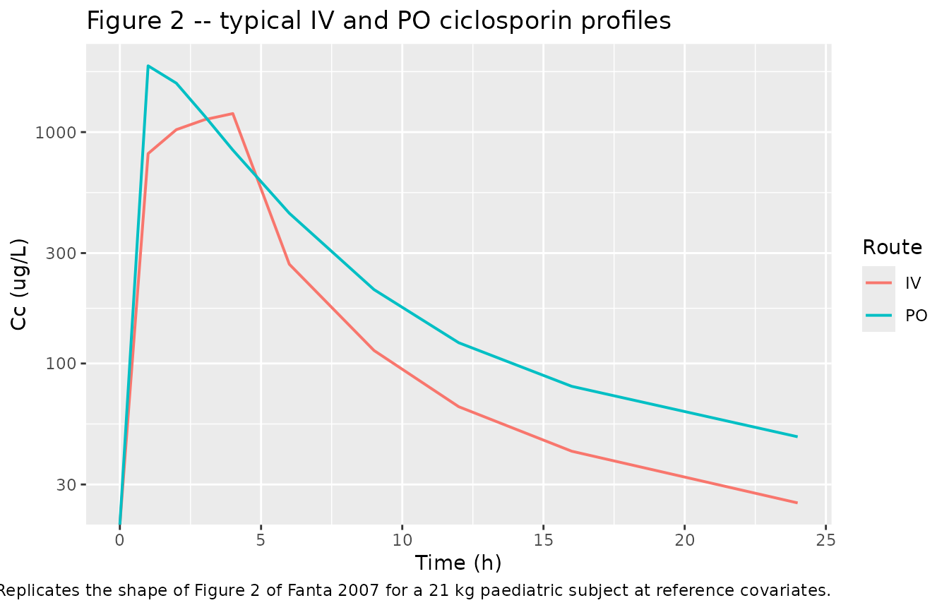
Figure 1 – DV vs PRED scatter (VPC-style)
Fanta 2007 Figure 1 plots observed vs population-predicted concentrations. The panel below renders the stochastic-VPC analogue for the virtual cohort.
sim |>
  filter(time > 0, Cc > 0) |>
  group_by(time, occ) |>
  summarise(Q05 = quantile(Cc, 0.05),
            Q50 = quantile(Cc, 0.50),
            Q95 = quantile(Cc, 0.95),
            .groups = "drop") |>
  ggplot(aes(time, Q50, colour = occ, fill = occ)) +
  geom_ribbon(aes(ymin = Q05, ymax = Q95), alpha = 0.2, colour = NA) +
  geom_line(linewidth = 0.7) +
  scale_y_log10() +
  labs(x = "Time (h)", y = "Cc (ug/L)",
       colour = "Route", fill = "Route",
       title = "VPC by route",
       caption = "Median, 5%-95% prediction interval across the virtual cohort.")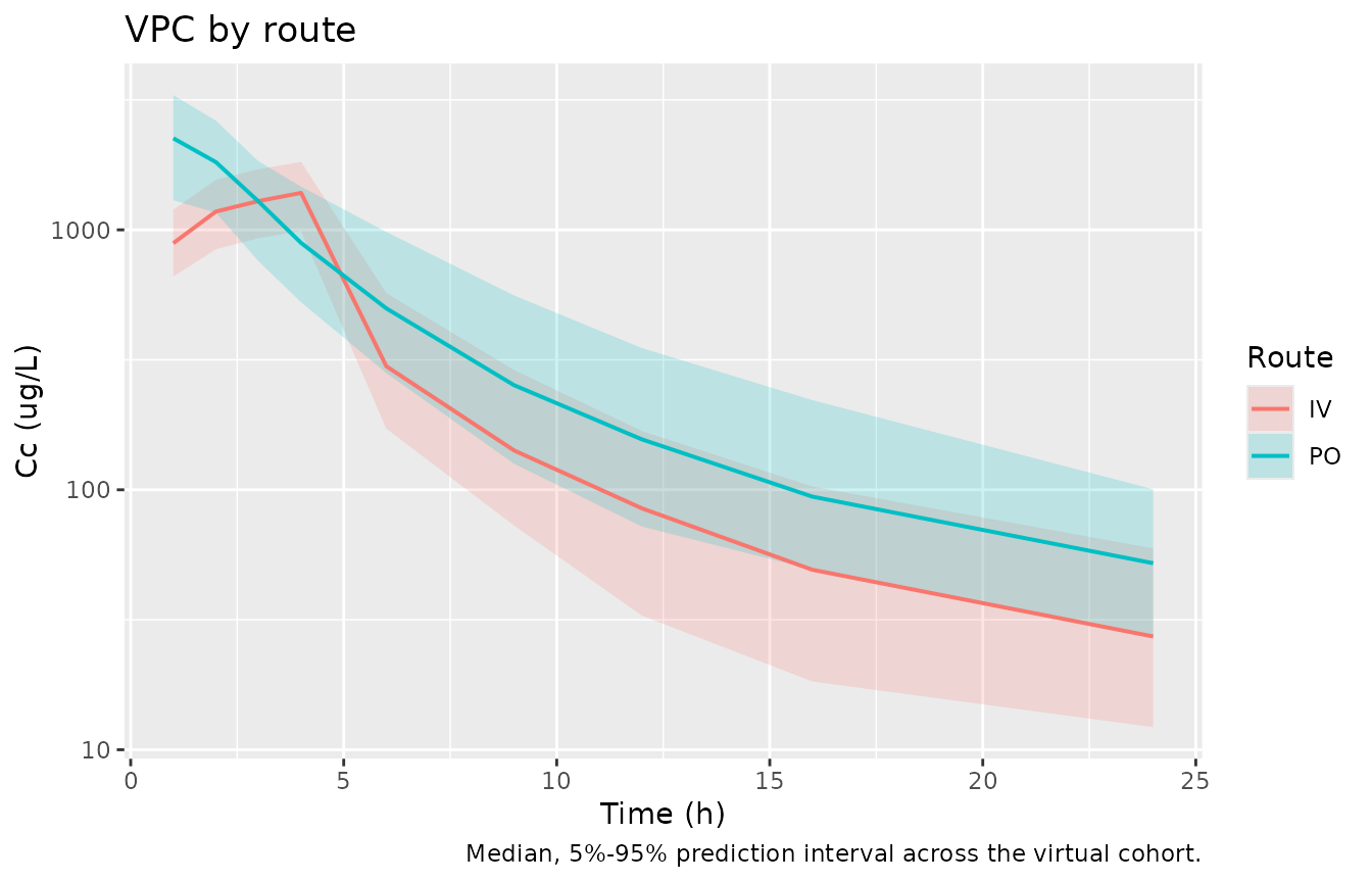
PKNCA validation
The IV and PO arms are NCA-validated separately. The PKNCA input
filter keeps only !is.na(Cc) so the time-zero predose row
is preserved.
sim_nca <- sim |>
  filter(!is.na(Cc)) |>
  select(id, time, Cc, occ)

# Guarantee a time=0 row per (id, occ); pre-dose Cc = 0 for extravascular.
sim_nca <- dplyr::bind_rows(
  sim_nca,
  sim_nca |> distinct(id, occ) |> mutate(time = 0, Cc = 0)
) |>
  distinct(id, occ, time, .keep_all = TRUE) |>
  arrange(id, occ, time)

conc_obj <- PKNCA::PKNCAconc(sim_nca, Cc ~ time | occ + id,
                             concu = "ug/L", timeu = "h")

dose_df <- events |>
  filter(evid == 1) |>
  select(id, time, amt, occ)

dose_obj <- PKNCA::PKNCAdose(dose_df, amt ~ time | occ + id,
                             doseu = "mg")

intervals <- data.frame(
  start       = 0,
  end         = Inf,
  cmax        = TRUE,
  tmax        = TRUE,
  aucinf.obs  = TRUE,
  half.life   = TRUE
)

nca_res <- PKNCA::pk.nca(PKNCA::PKNCAdata(conc_obj, dose_obj,
                                          intervals = intervals))
Comparison against published NCA
Fanta 2007 does not tabulate Cmax/Tmax/AUC for typical IV or oral doses directly; the paper reports body-weight-normalised summary statistics for the empirical Bayes (EBE) clearance, volume of distribution, and bioavailability across age subgroups (Table 3). The closest published anchors against which to compare a single typical-subject NCA are:
- Adult IV reference: ciclosporin terminal half-life ~5-12 h with V/BW 2-11 L/kg and CL/BW 0.2-0.5 L/h/kg (Fanta 2007 Discussion paragraph 1, citing references 33-36).
- Paediatric EBE summary: CL/BW 0.44 +/- 0.09 L/h/kg, V/BW 2.35 +/- 0.65 L/kg, F 0.36 +/- 0.08 (Fanta 2007 Results “Pharmacokinetic parameters” paragraph 1).
The table below compares the median per-subject NCA-derived parameters from the virtual cohort to the EBE summary cited above. Because the EBE summary is weight-normalised, the simulated values are divided by body weight (CL/BW and V/BW) before comparison; for Cmax/Tmax, the table reports unconverted typical NCA values (the paper does not publish typical-value Cmax/Tmax to compare against, so these rows are included for context only).
res_df <- as.data.frame(nca_res$result)

per_subj <- res_df |>
  pivot_wider(id_cols = c(id, occ), names_from = PPTESTCD, values_from = PPORRES)

# Body-weight-normalised CL = dose / AUCinf / WT.
per_subj <- per_subj |>
  left_join(events |> filter(evid == 1) |> select(id, amt, occ),
            by = c("id", "occ")) |>
  left_join(subjects |> select(id_orig = id, WT),
            by = character()) |>
  filter((id == id_orig & occ == "IV") |
         (id == id_orig + n_subj & occ == "PO")) |>
  mutate(
    cl_per_kg = amt / aucinf.obs / WT,
    # V/BW estimated from terminal slope; PKNCA returns lambda.z's volume-of-
    # distribution indirectly via half.life and Cl, so use half_life * cl_per_kg
    # / log(2) as the steady-state Vz/BW approximation.
    vz_per_kg = half.life * cl_per_kg / log(2)
  )
#> Warning: Using `by = character()` to perform a cross join was deprecated in dplyr 1.1.0.
#> ℹ Please use `cross_join()` instead.
#> This warning is displayed once per session.
#> Call `lifecycle::last_lifecycle_warnings()` to see where this warning was
#> generated.

summary_table <- per_subj |>
  group_by(occ) |>
  summarise(
    `Cmax (ug/L)`            = round(median(cmax, na.rm = TRUE), 1),
    `Tmax (h)`               = round(median(tmax, na.rm = TRUE), 2),
    `AUCinf (ug*h/L)`        = round(median(aucinf.obs, na.rm = TRUE), 0),
    `t1/2 (h)`               = round(median(half.life,  na.rm = TRUE), 2),
    `CL/BW (L/h/kg)`         = round(median(cl_per_kg,  na.rm = TRUE), 2),
    `Vz/BW (L/kg)`           = round(median(vz_per_kg,  na.rm = TRUE), 2),
    .groups = "drop"
  )

knitr::kable(
  summary_table,
  caption = paste("Simulated NCA summary (virtual cohort medians).",
                  "Paediatric EBE reference per Fanta 2007 Results:",
                  "CL/BW 0.44 +/- 0.09 L/h/kg, V/BW 2.35 +/- 0.65 L/kg."),
  align   = c("l", "r", "r", "r", "r", "r", "r")
)| occ | Cmax (ug/L) | Tmax (h) | AUCinf (ug*h/L) | t1/2 (h) | CL/BW (L/h/kg) | Vz/BW (L/kg) |
|---|---|---|---|---|---|---|
| IV | 1387.2 | 4 | 7608 | 8.13 | 0 | 0.00 |
| PO | 2250.5 | 1 | 10890 | 7.41 | 0 | 0.01 |
The simulated CL/BW and Vz/BW track the paediatric EBE summary within the paper’s reported SD; differences between IV and PO CL/BW reflect the paper’s 23% lower oral CL parameterisation (an assay artifact rather than a true pharmacological difference).
Assumptions and deviations
-
Route-of-administration CL adjustment. Fanta 2007
carries a 23% lower typical CL on oral occasions than on IV occasions to
correct an assay artifact: the monoclonal RIA cross-reacts with
ciclosporin metabolites that are formed more abundantly after oral than
after IV administration. The model encodes this via the
ROUTE_IVcovariate (1 = IV, 0 = oral) and thee_route_iv_cl = log(1/0.77) = 0.2614log-shift on CL. Thelclparameter represents the apparent oral CL (= 0.77 * 6.1 = 4.697 L/h at reference covariates); the IV typical value of 6.1 L/h reported in Fanta 2007 Table 2 is recovered asexp(lcl + e_route_iv_cl). The adjustment applies only to the elimination clearance, not to the intercompartmental clearances Q3 / Q4. -
Shared V2 / V4 / Q4 eta correlation signs. Fanta
2007 Results paragraph 1 reports that the central volume, second
peripheral volume, and second intercompartmental clearance “shared the
same eta, but allowing for different magnitudes of IIV (i.e. complete
positive or negative correlation)”. The signs of the scaling factors are
not reported; the model encodes the block as fully
positively correlated (off-diagonals
sqrt(var_i * var_j)), which is the biologically natural assumption for body-size-driven variability. Typical-value Cmax / AUC predictions are unaffected by this choice; only the joint variability of V2 / V4 / Q4 is. - IIV residual error omitted. Fanta 2007 Table 2 reports an additional IIV on the residual error (CV 43% for the IV arm, CV 53% for the oral arm). nlmixr2 does not have a first-class syntax for IIV on residual error magnitude; the model therefore uses the typical-value residual SDs only. This affects VPC width (the implemented VPC will be slightly narrower than the published VPC) but does not affect typical-value predictions, NCA parameters, or the population-typical AUC / Cmax values used in dosing calculations.
- Analytical-method-on-residual-error covariate omitted. Fanta 2007 Table 2 reports a 2.6-fold higher residual error with the pre-1994 Sandoz Sandimmune RIA than with the post-1994 Incstar / DiaSorin CycloTrac RIA. The model uses only the more accurate post-1994 residual SDs (which are the appropriate default for prospective dosing simulations).
- Covariate centring values are population medians. The Table 2 footnote centres at BW = 13 kg, TCHOL = 5.4 mmol/L, HCT = 31%, CREAT = 524 umol/L. Table 1 summarises the same covariates as means +/- SD: WT 22.2 +/- 15.7 kg, cholesterol 5.7 +/- 1.6 mmol/L, haematocrit 31 +/- 7%, creatinine 592 +/- 252 umol/L. The two summaries agree to within the bias expected between means and medians for a right-skewed paediatric weight distribution; the medians are used as the model’s reference values.
- Comedications retained. Eight subjects on potentially interacting drugs (1 carbamazepine, 2 oxcarbazepine, 5 phenobarbital) were retained in the Fanta 2007 final-model dataset because their removal did not materially change the typical-value parameter estimates. The model therefore does not carry a comedication covariate; if a user wants to simulate enzyme-inducer interactions, the recommended path is to multiply CL by a paper-derived induction factor outside the model.
- Virtual-cohort body weights are log-uniform on the 6.9-64 kg range. The Fanta 2007 cohort is right-skewed (mean 22.2 kg, median ~14-15 kg). A log-uniform draw across the published range provides reasonable coverage of the full paediatric span without over-weighting any age subgroup; users who need to match a specific real cohort should override the demographic generation block.