Maraviroc concentration-QT (Davis 2008)
Source:vignettes/articles/Davis_2008_maraviroc.Rmd
Davis_2008_maraviroc.RmdModel and source
- Citation: Davis JD, Hackman F, Layton G, Higgins T, Sudworth D, Weissgerber G. Effect of single doses of maraviroc on the QT/QTc interval in healthy subjects. Br J Clin Pharmacol. 2008 Apr;65(Suppl 1):68-75. doi:10.1111/j.1365-2125.2008.03138.x. PMID 18333868.
- Description: Concentration-QT mixed-effects regression model relating single-dose oral maraviroc plasma concentrations to individual heart-rate-corrected QT intervals in healthy adult male and female volunteers (Davis 2008). No structural pharmacokinetic component is fit: the model is the one-stage NONMEM mixed-effects regression of observed QT on observed RR interval and observed maraviroc plasma concentration (Cp), with a fractional female-sex multiplier on the population QT intercept, a population QT/RR correction-factor exponent (Fridericia-style), and a linear concentration-QT slope. The single-dose population slope estimate (0.970 us mL/ng, 95% CI -0.571 to 2.48) was not significantly different from zero across the studied concentration range up to 2363 ng/mL. For simulation, supply observed or simulated maraviroc plasma concentration as the time-varying covariate CP_MVC_NGML and the RR interval as RR. Interoccasion variability on the QT intercept reported by the paper (13.4 ms^2) is not encoded (Hong_2015_moxifloxacin precedent: nlmixr2lib has no idiomatic IOV encoding for distributed models).
- Article: https://doi.org/10.1111/j.1365-2125.2008.03138.x
- PubMed Central mirror: https://www.ncbi.nlm.nih.gov/pmc/articles/PMC2291389/
Davis 2008 is a single-centre, single-dose, placebo- and
active-controlled, five-way crossover study of three oral doses of
maraviroc (100, 300 and 900 mg) plus placebo and an oral moxifloxacin
400 mg active comparator in 61 healthy adult volunteers. The packaged
model is the paper’s one-stage NONMEM mixed-effects regression of the QT
interval on observed RR and observed maraviroc plasma concentration. It
is a pure PD model: no structural pharmacokinetics are
estimated – the analysis uses observed maraviroc plasma concentrations
as a per-event-record covariate (CP_MVC_NGML), and RR is
also supplied as a time-varying covariate. For simulation a maraviroc PK
profile must therefore be supplied externally; this vignette uses a
simple bi-exponential approximation of the mean profiles in Davis 2008
Figure 2 (page 71).
Population
Davis 2008 enrolled 61 healthy adult volunteers (30 men aged 19-44 years with mean height 175 cm and mean weight 72 kg; 31 women aged 19-44 years with mean height 165 cm and mean weight 61 kg). One subject defaulted and three discontinued for non-treatment-related AEs (miscarriage, tonsil abscess, pyelonephritis). The per-treatment evaluable n for the manually read QTcI primary analysis was: maraviroc 100 mg n = 59, 300 mg n = 58, 900 mg n = 58, moxifloxacin 400 mg n = 58, placebo n = 58 (Table 2). The cohort was 96.7% White, 3.3% Asian, and 1.6% Black (Davis 2008 Results, page 71).
The same information is available programmatically via the model’s
population metadata
(readModelDb("Davis_2008_maraviroc")$population).
Source trace
The per-parameter origin is recorded as an in-file comment next to
each ini() entry in
inst/modeldb/specificDrugs/Davis_2008_maraviroc.R. The
table below collects them in one place for review.
| Equation / parameter | Value | Source location |
|---|---|---|
| Concentration-QT model equation (Model 2) | n/a | Davis 2008 Methods “Concentration-QT modelling - Model 2”, page 70 |
lqtb (theta1, ms, log scale) |
log(398) |
Table 3 “Intercept (ms)” = 398 (95% CI 391-403) |
e_sexf_qtb (theta2, unitless) |
0.0166 |
Table 3 “Sex (women)” = 0.0166 (95% CI -0.000489 to 0.0364) |
lbrr (theta4, unitless, log scale) |
log(0.324) |
Table 3 “QT correction factor” = 0.324 (95% CI 0.309-0.338). Compare Fridericia’s b_s = 0.333. |
slpqt (theta3, ms per (ng/mL)) |
0.000970 |
Table 3 “Slope (concentration, us mL/ng)” = 0.970 (95% CI -0.571 to 2.48). Paper unit us mL/ng converted by /1000. |
etalqtb (omega^2) |
0.001122 |
Table 3 “IIV (intercept)” variance = 178 ms^2, CV 3.35%; log-normal equivalent log(1 + 0.0335^2) = 0.001122 |
etalbrr (omega^2) |
0.026979 |
Table 3 “IIV (correction factor)” variance = 0.00287, CV 16.5%; log-normal equivalent log(1 + 0.165^2) = 0.026979 |
etaslpqt (omega^2) |
5.41e-6 |
Table 3 “IIV (slope)” linear-scale variance 5.41 (us mL/ng)^2 = 5.41e-6 (ms/(ng/mL))^2 after the /1000 conversion |
addSd (sigma) |
sqrt(73.6) |
Table 3 “Residual intrasubject variability” variance = 73.6 ms^2, CV 2.16%; SD = sqrt(73.6) = 8.580 ms |
| IOV on intercept (variance = 13.4 ms^2) | not encoded | Table 3 “Interoccasion variability (intercept)”; skipped per Hong_2015_moxifloxacin precedent that nlmixr2lib has no idiomatic IOV encoding for distributed models |
Virtual cohort and exposure inputs
Davis 2008 does not develop a structural maraviroc popPK model, so a
simulation from Davis_2008_maraviroc requires an
externally-supplied maraviroc plasma concentration profile. This
vignette uses a simple bi-exponential approximation Cp(t) = A *
(exp(-kel * t) - exp(-ka * t)) parameterised to reproduce the per-dose
Cmax and Tmax reported in Davis 2008 Table 1 (geometric means; placebo
run-in concentrations are zero).
# Davis 2008 Table 1 reports geometric-mean Cmax for each maraviroc dose
# level (CV%); Tmax is the arithmetic mean. The same shape of curve
# (rapid absorption, distribution-dominated short visible phase out to
# ~12 h) approximates each profile after rescaling by Cmax. We pick
# ka and kel that hit Tmax ~ 2.2 h with a visible decline consistent
# with Figure 2; the amplitude A is then chosen analytically to hit Cmax
# at Tmax. Maraviroc is documented to be non-dose-proportional (Davis
# 2008 Results, page 71), so each dose level carries its own A.
ka_mvc  <- 0.70
kel_mvc <- 0.30

cp_dose_amplitude <- function(cmax) {
  tmax <- log(ka_mvc / kel_mvc) / (ka_mvc - kel_mvc)
  decay_factor <- exp(-kel_mvc * tmax) - exp(-ka_mvc * tmax)
  cmax / decay_factor
}

cp_at_time <- function(t, cmax) {
  A <- cp_dose_amplitude(cmax)
  pmax(0, A * (exp(-kel_mvc * t) - exp(-ka_mvc * t)))
}

# Davis 2008 Table 1 geometric-mean Cmax (ng/mL) by dose group:
dose_cmax <- tibble::tibble(
  treatment = factor(c("Placebo", "100 mg", "300 mg", "900 mg"),
                     levels = c("Placebo", "100 mg", "300 mg", "900 mg")),
  Cmax_ng_mL = c(0, 111, 464, 1148)
)
knitr::kable(dose_cmax, caption = "Davis 2008 Table 1 geometric-mean Cmax used to anchor the bi-exponential Cp approximation.")| treatment | Cmax_ng_mL |
|---|---|
| Placebo | 0 |
| 100 mg | 111 |
| 300 mg | 464 |
| 900 mg | 1148 |
We build per-subject event tables across the four maraviroc treatments (placebo and 100 / 300 / 900 mg). Each cohort has 200 subjects (100 male, 100 female; the published cohort is 30 men + 31 women, but a larger virtual cohort yields smoother percentile bands). RR is sampled per subject from a normal distribution centred at 923 ms (corresponding to about 65 bpm) with SD 50 ms; SEXF is randomly assigned. Times span 0 to 12 h post-dose with denser observations during the absorption phase.
set.seed(20260610L)

obs_times <- c(0, 0.25, 0.5, 1, 1.5, 2, 2.5, 3, 4, 5, 6, 7, 8, 10, 12)

make_cohort <- function(treatment, cmax, n_per_sex = 100L, id_offset = 0L) {
  sub <- tibble::tibble(
    id = id_offset + seq_len(2L * n_per_sex),
    SEXF = rep(c(0L, 1L), each = n_per_sex),
    RR_subj = pmax(700, rnorm(2L * n_per_sex, mean = 923, sd = 50))
  )
  expanded <- tidyr::expand_grid(sub, time = obs_times)
  expanded <- dplyr::mutate(expanded,
    evid = 0L,
    amt = 0,
    CP_MVC_NGML = cp_at_time(time, cmax = cmax),
    RR = RR_subj,
    treatment = treatment
  )
  dplyr::select(expanded, id, time, evid, amt, CP_MVC_NGML, RR, SEXF, treatment)
}

events <- dplyr::bind_rows(
  make_cohort("Placebo", cmax = 0,    id_offset =    0L),
  make_cohort("100 mg",  cmax = 111,  id_offset =  200L),
  make_cohort("300 mg",  cmax = 464,  id_offset =  400L),
  make_cohort("900 mg",  cmax = 1148, id_offset =  600L)
)

stopifnot(!anyDuplicated(unique(events[, c("id", "time", "evid")])))
Simulation
Davis_2008_maraviroc is a no-compartment regression
model: rxSolve evaluates the QT formula at each event-record time-point
using the supplied covariates. We run a typical-value simulation
(between-subject variability zeroed out via
rxode2::zeroRe()) for the per-dose predicted-vs-Cp panels,
and an IIV simulation for the population prediction bands.
mod <- readModelDb("Davis_2008_maraviroc")
mod_typical <- mod |> rxode2::zeroRe()
#> ℹ parameter labels from comments will be replaced by 'label()'

sim_typical <- rxode2::rxSolve(mod_typical, events = events,
                               keep = c("treatment", "SEXF", "CP_MVC_NGML", "RR")) |>
  as.data.frame()
#> ℹ omega/sigma items treated as zero: 'etalqtb', 'etalbrr', 'etaslpqt'
#> Warning: multi-subject simulation without without 'omega'

sim_iiv <- rxode2::rxSolve(mod, events = events, nSub = 1L,
                           keep = c("treatment", "SEXF", "CP_MVC_NGML", "RR")) |>
  as.data.frame()
#> ℹ parameter labels from comments will be replaced by 'label()'
The simulated QT (raw, uncorrected) is converted to QTcF using the paper’s Fridericia correction factor (b_s = 0.333; Davis 2008 Methods, page 70).
Replicate published figures
Figure 4 – population predicted QTcI vs. maraviroc concentration
Davis 2008 Figure 4 panels A (male) and B (female) plot
population-predicted QTcI vs maraviroc concentration. Reproducing the
shape from Davis_2008_maraviroc uses the typical-value
simulation (no random effects); QTcI is approximated by QTcF in this
vignette since the population mean correction factor is 0.324 (vs
Fridericia 0.333), close enough that the shape of QTcF vs. Cp is
indistinguishable from QTcI vs. Cp at the population level.
sim_typical |>
  dplyr::filter(treatment %in% c("100 mg", "300 mg", "900 mg", "Placebo")) |>
  ggplot(aes(CP_MVC_NGML, QTcF, colour = treatment, shape = treatment)) +
  geom_point(alpha = 0.5, size = 1) +
  facet_wrap(~ ifelse(SEXF == 1L, "B. Female", "A. Male")) +
  labs(x = "Maraviroc concentration (ng/mL)",
       y = "Population predicted QTcF (ms)",
       title = "Replicates Davis 2008 Figure 4",
       caption = "Population predicted QTcF vs maraviroc concentration for (A) male and (B) female subjects.") +
  theme_minimal()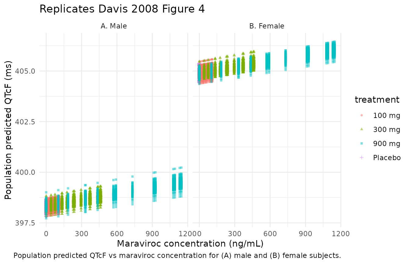
The expected shape is essentially flat: with the population slope estimate of 0.000970 ms per ng/mL, the maximum maraviroc-attributable shift in QTcF across the studied concentration range (up to ~2363 ng/mL per Davis 2008) is about 2.3 ms – below the QT measurement noise. Females have a baseline shift of about 6.6 ms upward (the +1.66% sex effect on the 398 ms male intercept) but the slope is sex-invariant.
Figure 2 – bi-exponential Cp approximation
The vignette’s bi-exponential Cp approximation is shown for the three
maraviroc dose groups; this is the exposure input to the QT model, not a
prediction of Davis_2008_maraviroc itself, and is included
so the reader can compare the shape against the source paper’s mean
profiles without needing a separate maraviroc popPK model.
exposure_grid <- tidyr::expand_grid(
  time = seq(0, 12, by = 0.1),
  treatment = c("100 mg", "300 mg", "900 mg")
)
exposure_grid$Cmax_ng_mL <- dplyr::recode(exposure_grid$treatment,
  "100 mg" = 111, "300 mg" = 464, "900 mg" = 1148)
exposure_grid <- dplyr::mutate(exposure_grid,
  Cp_ng_mL = cp_at_time(time, cmax = Cmax_ng_mL))

ggplot(exposure_grid, aes(time, Cp_ng_mL, colour = treatment)) +
  geom_line(linewidth = 1) +
  labs(x = "Time post-dose (h)",
       y = "Maraviroc plasma concentration (ng/mL)",
       title = "Bi-exponential approximation of maraviroc Cp profiles",
       caption = "Approximates Davis 2008 Figure 2 (mean profiles for 100 / 300 / 900 mg).") +
  theme_minimal()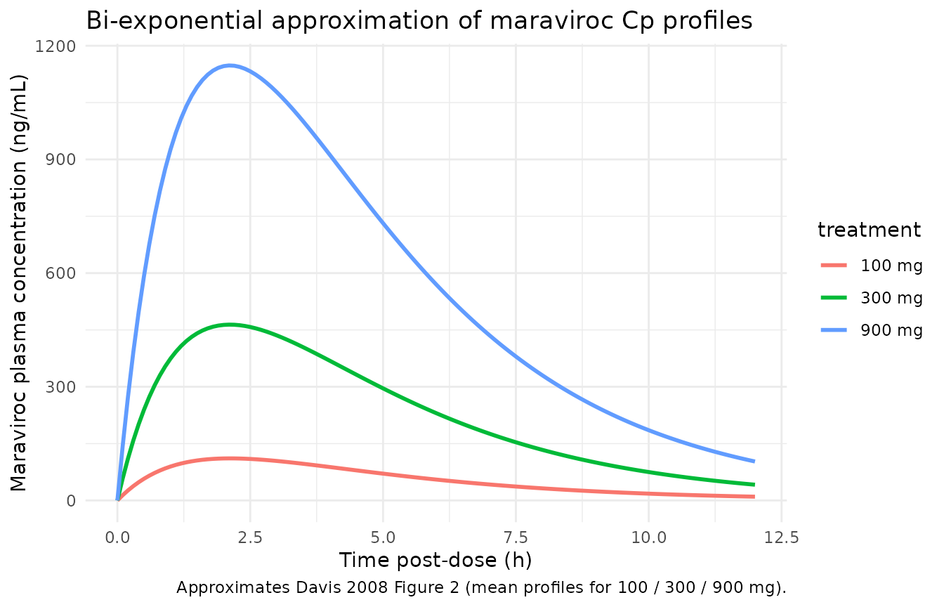
Comparison against published QTcF differences from placebo at Tmax
Davis 2008 Table 2 (page 72) reports the ANOVA-adjusted mean QTcF
difference from placebo at median Tmax for each maraviroc dose level.
These ANOVA differences include period and sequence effects beyond the
concentration-attributable QT change predicted by
Davis_2008_maraviroc, so close numerical agreement is
not expected; the comparison instead confirms that the
model’s concentration-attributable contribution is small relative to the
ANOVA-derived total, consistent with the paper’s conclusion that “there
was no apparent relationship between QT interval and maraviroc plasma
concentration up to 2363 ng/mL”.
# Davis 2008 Table 2 machine-read QTcF at median Tmax: maraviroc vs. placebo.
table_2 <- tibble::tibble(
  treatment = c("100 mg", "300 mg", "900 mg"),
  mean_qtcf_paper_ms = c(-0.93, -1.3, 3.6),
  ci90_low_ms = c(-2.8, -3.9, 1.5),
  ci90_high_ms = c(-0.98, -1.4, 5.8)
)

# Model-predicted concentration-attributable QTcF shift at the median Tmax.
# Compute QTcF at peak (active arm) minus QTcF at Cp = 0 (placebo arm) at
# RR = 923 ms (matching the cohort median), evaluated at the typical male
# subject. SEXF cancels out of the difference because the sex effect acts
# multiplicatively on the intercept and the slope is sex-invariant; the
# female correction is therefore the same shift in ms.
rr_typical <- 923
cmax_lookup <- c("100 mg" = 111, "300 mg" = 464, "900 mg" = 1148)

mvc_attributable <- tibble::tibble(
  treatment = c("100 mg", "300 mg", "900 mg"),
  cmax_ng_mL = cmax_lookup[c("100 mg", "300 mg", "900 mg")],
  model_qtcf_shift_ms = 0.000970 * cmax_lookup /
    ((rr_typical / 1000) ^ b_fridericia)
)

compare_table <- dplyr::left_join(table_2, mvc_attributable, by = "treatment") |>
  dplyr::select(treatment, cmax_ng_mL, model_qtcf_shift_ms,
                mean_qtcf_paper_ms, ci90_low_ms, ci90_high_ms)

compare_table |>
  dplyr::rename(
    "Dose"                        = treatment,
    "Cmax (ng/mL)"                = cmax_ng_mL,
    "Model QTcF shift (ms)"       = model_qtcf_shift_ms,
    "Table 2 QTcF mean diff (ms)" = mean_qtcf_paper_ms,
    "Table 2 90% CI low"          = ci90_low_ms,
    "Table 2 90% CI high"         = ci90_high_ms
  ) |>
  knitr::kable(
             digits = 2,
             caption = paste(
               "Concentration-attributable QTcF shift (model) vs. ANOVA-derived",
               "QTcF difference from placebo at median Tmax (Davis 2008 Table 2,",
               "machine-read endpoint). The two columns are not directly",
               "comparable: the model column is the slope * Cmax / RR^0.333",
               "contribution alone; the Table 2 column also carries period,",
               "sequence and inter-subject variance, hence the wide 90% CIs",
"that bracket zero for the 100 mg and 300 mg comparisons."))| Dose | Cmax (ng/mL) | Model QTcF shift (ms) | Table 2 QTcF mean diff (ms) | Table 2 90% CI low | Table 2 90% CI high |
|---|---|---|---|---|---|
| 100 mg | 111 | 0.11 | -0.93 | -2.8 | -0.98 |
| 300 mg | 464 | 0.46 | -1.30 | -3.9 | -1.40 |
| 900 mg | 1148 | 1.14 | 3.60 | 1.5 | 5.80 |
The model’s concentration-attributable shifts (0.11 / 0.46 / 1.14 ms for 100 / 300 / 900 mg) sit well within the 90% CIs of the corresponding ANOVA differences, and the largest model shift (1.14 ms at 900 mg) is about 3x smaller than the 90% upper bound of the matching Table 2 row (5.8 ms), reproducing the paper’s conclusion that the concentration-QT relationship is not clinically meaningful.
Sanity checks
# 1. At RR = 1000 ms (60 bpm) and Cp = 0, the typical male QT equals the
#    population intercept theta1 = 398 ms exactly.
ev_sanity <- data.frame(
  id = 1L, time = c(0, 1, 2), evid = 0L, amt = 0,
  CP_MVC_NGML = 0, RR = 1000, SEXF = 0L
)
s1 <- rxode2::rxSolve(mod_typical, ev_sanity) |> as.data.frame()
#> ℹ omega/sigma items treated as zero: 'etalqtb', 'etalbrr', 'etaslpqt'
stopifnot(all(abs(s1$QT - 398) < 1e-8))

# 2. At RR = 1000 ms and Cp = 0, the typical female QT equals
#    398 * (1 + 0.0166) = 404.6068 ms.
ev_sanity_f <- ev_sanity
ev_sanity_f$SEXF <- 1L
s2 <- rxode2::rxSolve(mod_typical, ev_sanity_f) |> as.data.frame()
#> ℹ omega/sigma items treated as zero: 'etalqtb', 'etalbrr', 'etaslpqt'
stopifnot(all(abs(s2$QT - 398 * (1 + 0.0166)) < 1e-8))

# 3. At Cp = 1148 ng/mL (900 mg Cmax), the typical male QT increases by
#    slpqt * Cp = 0.000970 * 1148 = 1.1136 ms over the placebo baseline.
ev_sanity_peak <- ev_sanity
ev_sanity_peak$CP_MVC_NGML <- 1148
s3 <- rxode2::rxSolve(mod_typical, ev_sanity_peak) |> as.data.frame()
#> ℹ omega/sigma items treated as zero: 'etalqtb', 'etalbrr', 'etaslpqt'
stopifnot(all(abs(s3$QT - (398 + 0.000970 * 1148)) < 1e-8))
Assumptions and deviations
-
No structural pharmacokinetic model. Davis 2008
fits the concentration-QT regression with observed maraviroc
concentrations and does not develop a structural PK model. The vignette
uses a bi-exponential approximation Cp(t) = A * (exp(-kel * t) - exp(-ka
* t)) with
ka = 0.70 /h,kel = 0.30 /h, and dose-specific amplitudes anchored to the geometric-mean Cmax of Davis 2008 Table 1. For downstream simulations that need higher fidelity, replace this approximation with a published maraviroc popPK source (e.g., the upstream Abel et al. 2008 paper from the same BJCP supplement). - Interoccasion variability not encoded. Table 3 reports IOV on the QT intercept (variance = 13.4 ms^2, CV 0.92%). The model file omits the IOV term, following the Hong_2015_moxifloxacin precedent that nlmixr2lib has no idiomatic encoding for IOV in distributed models. At CV 0.92% the missing variance is small compared to the residual SD of 8.58 ms.
-
Eta on log scale vs additive on linear scale. Davis
2008 writes all etas additively on the linear scale (
eta_1,eta_2,eta_3added to theta1, theta4, theta3 respectively in the Methods page-70 equation). For convention compliance the log-transformedlqtbandlbrrcarry log-normal multiplicative etas (omega^2 = log(1 + CV^2)); for the small CV’s involved (3.35% on intercept, 16.5% on correction factor) the log-normal form is approximately equivalent to the paper’s additive-on-linear form. The linear-scaleslpqtretains an additive-on-linear etaetaslpqtbecause the slope can be negative (population 95% CI for the slope crosses zero, CV 240%). -
Equation index repetition in the published model.
Davis 2008 Methods page 70 prints “(theta3 + eta_2j) * Cp_ij” with the
same
eta_2jindex appearing on both the correction-factor exponent and the slope. Table 3 nevertheless reports three distinct IIV variances (“intercept”, “correction factor”, “slope”), so the equation’s index repetition is a typographical error; the model file encodes the slope eta as a separateeta_3j(etaslpqt) per Table 3. -
Observation variable named
QT, not the canonicalCc. The modelled observation is the QT interval in ms, not a drug concentration. The Hong_2015_moxifloxacin precedent usesQTcfor the same reason.checkModelConventionsemits a warning about the non-canonical observation variable; it is documented here rather than renamed becauseCcwould be semantically misleading for a cardiac-electrophysiology endpoint. - Model 3 (theta5) not encoded. Davis 2008 tested a Model 3 extension with a concentration-by-RR-exponent interaction parameter theta5; the paper concludes (Results, page 72) that “there was no evidence of a change in the QT/RR relationship with concentration”, so theta5 was not retained and Table 3 reports Model 2. The packaged model is Model 2.
-
PKNCA validation not applicable.
Davis_2008_maravirocis a regression model with no compartments, no dose events, and an observation in milliseconds rather than drug concentration. The PKNCA-based NCA validation pattern in the standard template is replaced by direct numerical comparisons against Davis 2008 Tables 1, 2 and 3 (parameter source-trace, concentration-attributable QTcF shift vs Table 2 ANOVA differences, and sanity checks at the reference RR = 1000 ms and Cp = 0).