Treosulfan and EBDM in rat plasma and brain (Danielak 2020)
Source:vignettes/articles/Danielak_2020_treosulfan_rat.Rmd
Danielak_2020_treosulfan_rat.RmdModel and source
- Citation: Danielak D, Romanski M, Kasprzyk A, Tezyk A, Glowka F. Population pharmacokinetic approach for evaluation of treosulfan and its active monoepoxide disposition in plasma and brain on the basis of a rat model. Pharmacol Rep. 2020;72(5):1297-1309. doi:10.1007/s43440-020-00115-0. Correction: Pharmacol Rep. 2020;72:1443. doi:10.1007/s43440-020-00144-9 (units of the first-order rate constants corrected from L/h to 1/h; no values changed)
- Description: Preclinical (rat). Joint parent-metabolite population PK model for treosulfan (TREO) and its active monoepoxide (S,S)-1,2-epoxybutane-3,4-diol-4-methanesulfonate (EBDM) in plasma and brain of Wistar rats after a single 500 mg/kg intraperitoneal dose (Danielak 2020). First-order absorption into a one-compartment TREO plasma model; irreversible first-order conversion of TREO to EBDM (fixed rate constants in plasma and in brain); one-compartment EBDM plasma model; bidirectional blood-brain barrier transport of TREO and EBDM parameterised by an influx clearance and the influx/efflux clearance ratio; a second (deep) brain compartment for TREO. All clearances and volumes are apparent (divided by F) and per kg body weight. Male sex lowers TREO plasma clearance by 14.6%. IIV on ka and TREO CL; proportional residual error fixed to 15% (plasma) and 20% (brain).
- Article: https://doi.org/10.1007/s43440-020-00115-0 (open access)
- Correction: https://doi.org/10.1007/s43440-020-00144-9
Treosulfan is a prodrug: it converts non-enzymatically (pH- and temperature-dependent) to the active monoepoxide EBDM, and then to the diepoxide DEB. Danielak et al. fitted a joint parent-metabolite model to plasma and brain concentrations of treosulfan (TREO) and EBDM in Wistar rats to quantify blood-brain barrier (BBB) penetration.
Population
96 ten-week-old Wistar rats (48 male, 48 female; mean body weight 306 +/- 25 g for males and 188 +/- 15 g for females) received a single intraperitoneal dose of 500 mg/kg treosulfan (1797 umol/kg). The design was destructive (one animal per sampling time): plasma and brain were collected predose and at 0.25, 0.5, 1, 2, 4, 6 and 24 h. One female with an outlying 0.25 h plasma concentration was excluded, and the 24 h samples (all below the limit of quantitation) were dropped (Methods “Animals” and “Sample collection”, Fig. 2; Results first paragraph).
The same information is available programmatically via
readModelDb("Danielak_2020_treosulfan_rat")()$population.
Source trace
The per-parameter origin is recorded as an in-file comment next to
each ini() entry in
inst/modeldb/specificDrugs/Danielak_2020_treosulfan_rat.R.
All clearances and volumes are apparent (divided by the unknown
intraperitoneal bioavailability F) and per kg body weight.
| Equation / parameter | Value | Source location |
|---|---|---|
lka (k12) |
log(5.12) 1/h | Table 1 |
lcl (CL1/F, females) |
log(0.419) L/h/kg | Table 1 |
lvc (V2/F) |
fixed log(1.03) L/kg | Table 1 |
lkmet (k23, TREO to EBDM in plasma) |
fixed log(0.451) 1/h | Table 1; Methods assumption (4) |
lkmet_brain (k45, TREO to EBDM in brain) |
fixed log(0.271) 1/h | Table 1; Methods assumption (5), log10(kf) = -7.479 + 0.960 pH at pH 7.2 |
lcl_ebdm (CL2/F) |
log(6.24) L/h/kg | Table 1 |
lvc_ebdm (V3/F) |
fixed log(0.914) L/kg | Table 1 |
lclin (Q1/F, TREO BBB influx clearance) |
log(0.0233) L/h/kg | Table 1; Methods assumption (7) |
lkp_brain (BBB1 = CLin/CLout, TREO) |
log(0.120) | Table 1 |
lv_brain_extravascular (V4/F) |
fixed log(6.56e-3) L/kg | Table 1; Results “Prediction of treosulfan concentrations in brain” |
lq_brain_deep (Q2/F) |
log(0.304) L/h/kg | Table 1 |
lv_brain_deep (V6/F) |
fixed log(0.364) L/kg | Table 1 |
lclin_ebdm (Q3/F, EBDM BBB influx clearance) |
log(0.0122) L/h/kg | Table 1 |
lkp_brain_ebdm (BBB2 = CLin/CLout, EBDM) |
log(0.317) | Table 1 |
lv_brain_extravascular_ebdm (V5/F) |
fixed log(6.56e-3) L/kg | Table 1 |
e_sex_cl (COV CL-MALE) |
-0.146 | Table 1 and footnote a |
etalka |
0.38941 (69% CV) | Table 1, footnote b |
etalcl |
0.00995 (10% CV) | Table 1, footnote b |
propSd, propSd_ebdm
|
fixed 0.15 | Table 1; Methods “Population pharmacokinetic analysis” |
propSd_Cbrain, propSd_Cbrain_ebdm
|
fixed 0.20 | Table 1; Methods |
| Structure (six compartments, arrows) | n/a | Figure 3 |
clef = clin / kp_brain |
n/a | Methods assumption (7): BBB = CLin / CLout |
cl = tvcl * (1 + e_sex_cl * (1 - SEXF)) |
n/a | Table 1 footnote a |
Deterministic checks on the typical animal
The typical male and female are solved without random effects on a log-spaced early grid (absorption is fast, k12 = 5.12 1/h) out to 72 h so that the AUCs are essentially complete.
mod <- readModelDb("Danielak_2020_treosulfan_rat")
mod_typ <- rxode2::zeroRe(mod)
#> ℹ parameter labels from comments will be replaced by 'label()'
dose <- 1797 # umol/kg; 500 mg/kg / 278.29 g/mol (Methods)

grid <- sort(unique(c(0, 10^seq(-3, log10(72), length.out = 600))))
ev_typ <- dplyr::bind_rows(
  data.frame(id = 1L, time = 0, amt = dose, evid = 1L, cmt = "depot",
             dvid = NA_integer_, SEXF = 1),
  data.frame(id = 1L, time = grid, amt = 0, evid = 0L, cmt = "central",
             dvid = 1L, SEXF = 1),
  data.frame(id = 2L, time = 0, amt = dose, evid = 1L, cmt = "depot",
             dvid = NA_integer_, SEXF = 0),
  data.frame(id = 2L, time = grid, amt = 0, evid = 0L, cmt = "central",
             dvid = 1L, SEXF = 0)
)
sim_typ <- rxode2::rxSolve(mod_typ, events = ev_typ, rtol = 1e-10, atol = 1e-12,
                           maxsteps = 1e6, returnType = "data.frame")
#> ℹ omega/sigma items treated as zero: 'etalka', 'etalcl'
#> Warning: multi-subject simulation without without 'omega'
sim_typ$sex <- ifelse(sim_typ$id == 1, "Female", "Male")

trap <- function(t, y) sum(diff(t) * (head(y, -1) + tail(y, -1)) / 2)
auc_typ <- sim_typ |>
  dplyr::group_by(sex) |>
  dplyr::summarise(
    cl = cl[1], cl_ebdm = cl_ebdm[1],
    auc_treo = trap(time, Cc),
    auc_ebdm = trap(time, Cc_ebdm),
    auc_brain = trap(time, Cbrain),
    auc_brain_ebdm = trap(time, Cbrain_ebdm),
    c025 = Cc[which.min(abs(time - 0.25))],
    .groups = "drop"
  ) |>
  dplyr::mutate(
    recovered_pct = 100 * (cl * auc_treo + cl_ebdm * auc_ebdm) / dose,
    ratio_treo = auc_brain / auc_treo,
    ratio_ebdm = auc_brain_ebdm / auc_ebdm
  )
knitr::kable(auc_typ, digits = 4,
caption = "Typical-animal exposures (AUC in umol*h/L, CL in L/h/kg).")| sex | cl | cl_ebdm | auc_treo | auc_ebdm | auc_brain | auc_brain_ebdm | c025 | recovered_pct | ratio_treo | ratio_ebdm |
|---|---|---|---|---|---|---|---|---|---|---|
| Female | 0.4190 | 6.24 | 2033.518 | 151.4520 | 241.8083 | 59.1800 | 1108.299 | 100.0058 | 0.1189 | 0.3908 |
| Male | 0.3578 | 6.24 | 2184.750 | 162.7154 | 259.7914 | 63.5812 | 1118.068 | 100.0058 | 0.1189 | 0.3908 |
Three checks follow, all on deterministic quantities.
-
Mass balance. Every molecule of treosulfan leaves
the body either unchanged through CL1/F or, after conversion, as EBDM
through CL2/F (the brain compartments have no elimination of their own).
Therefore
CL1 * AUC(TREO, plasma) + CL2 * AUC(EBDM, plasma) = Dose. A wrong conversion or transfer term breaks this identity. - Sex effect. The typical male CL1/F must be 0.419 * (1 - 0.146) = 0.358 L/h/kg, the male median shown in Figure 6 of the paper.
-
Brain penetration of treosulfan. Integrating the
brain mass balance to infinity gives
AUC(brain) / AUC(plasma) = CLin / (CLout + k45 * V4)= 0.1189; the value is independent of sex and is close to BBB1 = 0.120 because conversion in the small brain volume is slow compared with efflux.
kin_ratio <- 0.0233 / (0.0233 / 0.120 + 0.271 * 6.56e-3)
stopifnot(
  nrow(auc_typ) == 2,
  all(abs(auc_typ$recovered_pct - 100) < 0.5),
  abs(auc_typ$cl[auc_typ$sex == "Male"] - 0.419 * (1 - 0.146)) < 1e-6,
  abs(auc_typ$cl[auc_typ$sex == "Female"] - 0.419) < 1e-6,
  all(abs(auc_typ$ratio_treo / kin_ratio - 1) < 0.01)
)
The paper that first analysed these same animals by naive pooling reported a brain-to-plasma AUC ratio of about 0.1 for treosulfan (Danielak 2020 Discussion, citing Romanski et al.); the model gives 0.119. EBDM penetrates better (typical AUC ratio 0.391), consistent with BBB2 = 0.317 plus local formation of EBDM from treosulfan inside the brain.
The mean plasma treosulfan concentration observed 0.25 h after dosing was 1147 uM (Results first paragraph, excluding the outlier); the typical-animal prediction at 0.25 h is 1108 uM (female) and 1118 uM (male).
Virtual cohort and simulation
Original data are not available. The cohort below is 100 males and
100 females dosed with 1797 umol/kg into the peritoneal depot, observed
on the paper’s sampling grid (0.25-6 h) plus a dense grid for the NCA.
The model has four error endpoints (Cc,
Cc_ebdm, Cbrain, Cbrain_ebdm), so
observation rows carry dvid = 1; every concentration is
still returned as a column.
set.seed(2020)
n_per_sex <- 100
obs_times <- sort(unique(c(0, 0.05, 0.1, 0.25, 0.5, 0.75, 1, 1.5, 2, 3, 4, 5, 6,
                           8, 10, 12, 16, 20, 24)))
make_cohort <- function(n, sexf, id_offset) {
  ids <- id_offset + seq_len(n)
  dplyr::bind_rows(
    data.frame(id = ids, time = 0, amt = dose, evid = 1L, cmt = "depot",
               dvid = NA_integer_),
    tidyr::expand_grid(id = ids, time = obs_times) |>
      dplyr::mutate(amt = 0, evid = 0L, cmt = "central", dvid = 1L)
  ) |>
    dplyr::mutate(SEXF = sexf, sex = ifelse(sexf == 1, "Female", "Male")) |>
    dplyr::arrange(id, time, dplyr::desc(evid))
}
events <- dplyr::bind_rows(
  make_cohort(n_per_sex, 1, 0L),
  make_cohort(n_per_sex, 0, n_per_sex)
)
stopifnot(!anyDuplicated(events[, c("id", "time", "evid")]))

rxode2::rxSetSeed(2020)
sim <- rxode2::rxSolve(mod, events = events, keep = "sex",
                       returnType = "data.frame")
#> ℹ parameter labels from comments will be replaced by 'label()'
Replicate Figure 5 (VPC)
# Replicates Figure 5 of Danielak 2020: 5th, 50th and 95th percentiles of the
# four measured analytes over the 0.25-6 h sampling window.
sim |>
  dplyr::filter(time >= 0.25, time <= 6) |>
  dplyr::select(id, time, sex, Cc, Cc_ebdm, Cbrain, Cbrain_ebdm) |>
  tidyr::pivot_longer(c(Cc, Cc_ebdm, Cbrain, Cbrain_ebdm),
                      names_to = "analyte", values_to = "conc") |>
  dplyr::mutate(analyte = factor(
    analyte,
    levels = c("Cc", "Cc_ebdm", "Cbrain", "Cbrain_ebdm"),
    labels = c("Treosulfan, plasma", "EBDM, plasma",
               "Treosulfan, brain", "EBDM, brain")
  )) |>
  dplyr::group_by(analyte, time) |>
  dplyr::summarise(
    Q05 = quantile(conc, 0.05), Q50 = median(conc), Q95 = quantile(conc, 0.95),
    .groups = "drop"
  ) |>
  ggplot(aes(time, Q50)) +
  geom_ribbon(aes(ymin = Q05, ymax = Q95), alpha = 0.3) +
  geom_line() +
  facet_wrap(~analyte, scales = "free_y") +
  scale_y_log10() +
  labs(x = "Time after dose (h)", y = "Concentration (uM)",
       caption = "Replicates Figure 5 of Danielak 2020 (90% prediction interval, median).")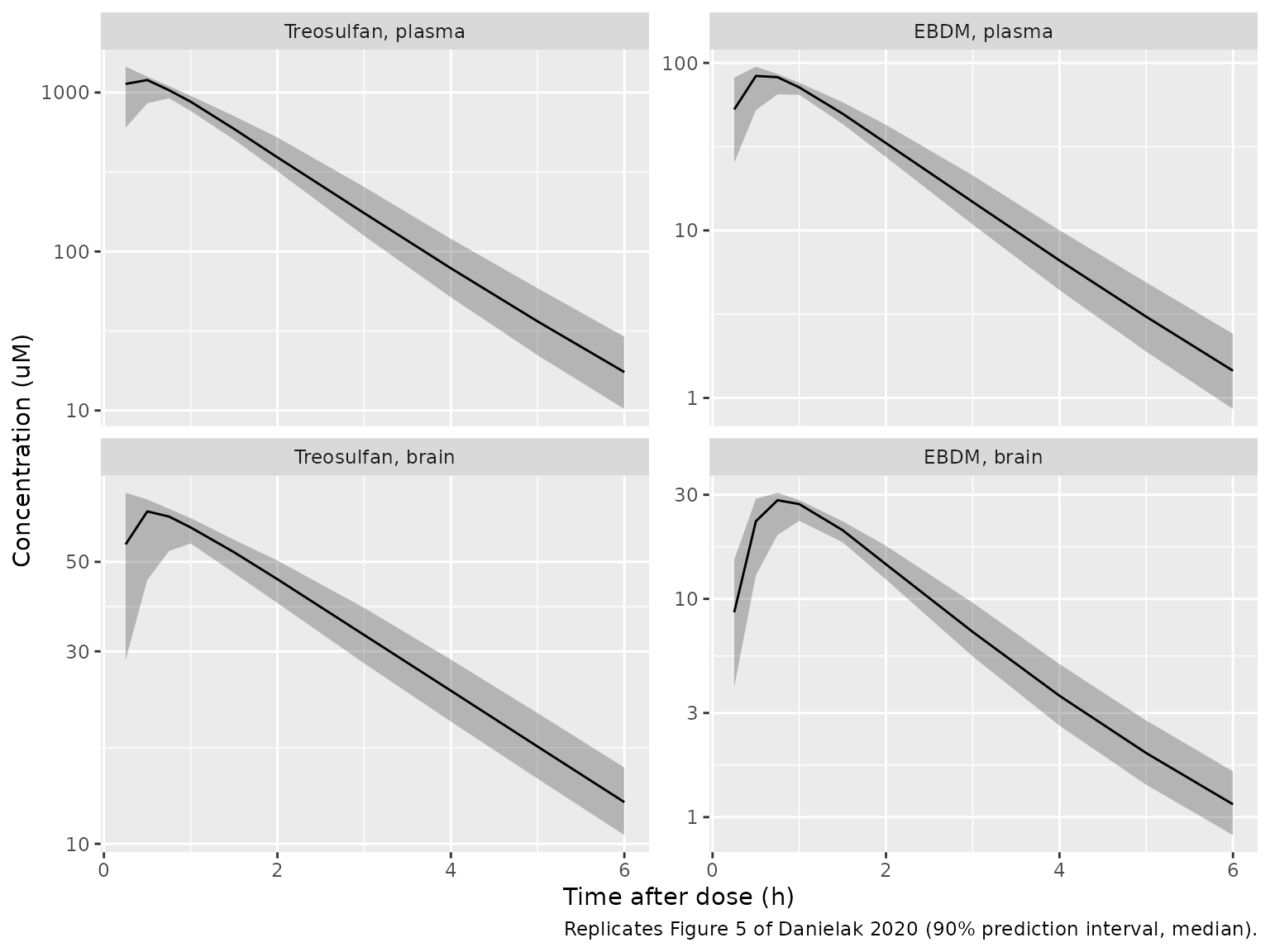
Replicate Figure 6 (clearance by sex)
cl_ind <- sim |>
  dplyr::distinct(id, sex, cl)
ggplot(cl_ind, aes(sex, cl)) +
  geom_boxplot() +
  labs(x = "Sex", y = "CL1/F (L/h/kg)",
       caption = "Replicates Figure 6 of Danielak 2020 (individual CL1/F by sex).")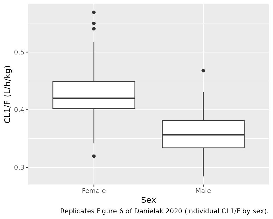
cl_med <- cl_ind |>
  dplyr::group_by(sex) |>
  dplyr::summarise(median_cl = median(cl), .groups = "drop")
knitr::kable(cl_med, digits = 3)| sex | median_cl |
|---|---|
| Female | 0.420 |
| Male | 0.357 |
# Figure 6 medians: about 0.358 (male) and 0.419 (female). With a 10% CV the
# median of 100 draws is within ~3% of the typical value; 8% still catches
# a sign error on e_sex_cl (0.48 vs 0.36 L/h/kg).
stopifnot(
  abs(cl_med$median_cl[cl_med$sex == "Male"] / 0.358 - 1) < 0.08,
  abs(cl_med$median_cl[cl_med$sex == "Female"] / 0.419 - 1) < 0.08
)
PKNCA validation
Plasma treosulfan NCA by sex. The paper does not report NCA values, so there is no published table to compare against; the checks above serve as the quantitative validation.
sim_nca <- sim |>
  dplyr::filter(!is.na(Cc)) |>
  dplyr::select(id, time, Cc, sex)
sim_nca <- dplyr::bind_rows(
  sim_nca,
  sim_nca |> dplyr::distinct(id, sex) |> dplyr::mutate(time = 0, Cc = 0)
) |>
  dplyr::distinct(id, sex, time, .keep_all = TRUE) |>
  dplyr::arrange(id, time)

conc_obj <- PKNCA::PKNCAconc(sim_nca, Cc ~ time | sex + id)
dose_df <- events |>
  dplyr::filter(evid == 1) |>
  dplyr::select(id, time, amt, sex)
dose_obj <- PKNCA::PKNCAdose(dose_df, amt ~ time | sex + id)
intervals <- data.frame(start = 0, end = Inf, cmax = TRUE, tmax = TRUE,
                        aucinf.obs = TRUE, half.life = TRUE)
nca_res <- PKNCA::pk.nca(PKNCA::PKNCAdata(conc_obj, dose_obj,
                                          intervals = intervals))
nca_sum <- as.data.frame(nca_res$result) |>
  dplyr::filter(PPTESTCD %in% c("cmax", "tmax", "aucinf.obs", "half.life")) |>
  dplyr::group_by(sex, PPTESTCD) |>
  dplyr::summarise(median = median(PPORRES, na.rm = TRUE), .groups = "drop") |>
  tidyr::pivot_wider(names_from = PPTESTCD, values_from = median)
nca_sum |>
  dplyr::rename(
    "Sex" = sex,
    "Cmax (uM)" = cmax,
    "Tmax (h)" = tmax,
    "AUC0-inf (uM*h)" = aucinf.obs,
    "t1/2 (h)" = half.life
  ) |>
knitr::kable(digits = 2, caption = "Median simulated plasma treosulfan NCA by sex.")| Sex | AUC0-inf (uM*h) | Cmax (uM) | t1/2 (h) | Tmax (h) |
|---|---|---|---|---|
| Female | 2012.83 | 1188.40 | 2.18 | 0.5 |
| Male | 2169.22 | 1225.87 | 2.18 | 0.5 |
# AUC0-inf does not depend on ka, and IIV on CL1/F is only 10% CV, so the
# cohort median must sit close to the typical-animal AUC computed above. A
# dose, unit or clearance error moves it by far more than 10%.
auc_m <- nca_sum$aucinf.obs[nca_sum$sex == "Male"]
auc_f <- nca_sum$aucinf.obs[nca_sum$sex == "Female"]
stopifnot(
  length(auc_m) == 1, length(auc_f) == 1,
  abs(auc_f / auc_typ$auc_treo[auc_typ$sex == "Female"] - 1) < 0.1,
  abs(auc_m / auc_typ$auc_treo[auc_typ$sex == "Male"] - 1) < 0.1
)
Assumptions and deviations
-
Abstract vs. Table 1 for male clearance. The
abstract gives the male CL1/F as 0.273 L/h/kg, which is 0.419 - 0.146
(the coefficient subtracted as an absolute value). Table 1 footnote a
defines the effect as fractional,
CL1-MALE/F = CL1/F + CL1/F * COV, giving 0.358 L/h/kg, and the male median in Figure 6 is 0.358. The model follows the footnote and Figure 6. - Units of the rate constants. The original online version printed the first-order rate constants in L/h; the Correction (doi:10.1007/s43440-020-00144-9) changes the units to 1/h without changing any value. The open-access article carries the corrected units.
-
Q1/F and Q3/F are the BBB influx clearances.
Methods assumption (7) parameterises BBB transport by the influx
clearance CLin and the ratio BBB = CLin / CLout; Figure 3 labels the
plasma-brain arrows Q1/F, BBB1 and Q3/F, BBB2. The model therefore uses
clin = Q/Fandclef = clin / BBB. - Brain treosulfan converts to EBDM only in the central brain compartment (k45), and there is no other brain elimination (Figure 3; Results “Blood- brain transport of treosulfan and EBDM”).
-
Brain observations are the central brain
compartments (V4/F for treosulfan, V5/F for EBDM), per Results
“Prediction of treosulfan concentrations in brain”. The deep brain
compartment (V6/F) is exposed as
Cbrain_deepbut was not observed. - Per-kg dosing. The paper specified the dose as 1797 umol/kg for every animal, so all volumes and clearances are per kg and no body-weight covariate is needed. Supply doses in umol/kg.
- Bioavailability. All parameters are apparent (/F); F was not identifiable and is implicitly 1.
- Residual error was fixed to the assay precision (15% plasma, 20% brain) because a one-animal-per-sample design cannot identify it.