Remimazolam (Ueshima 2025)
Source:vignettes/articles/Ueshima_2025_remimazolam.Rmd
Ueshima_2025_remimazolam.RmdModel and source
- Citation: Ueshima S, Nagahara S, Nakaya K, Kawamura M, Hira D, Matsuura Y, Toyama H, Kawamae K, Kakumoto M. Pharmacokinetic and pharmacodynamic characterization of remimazolam in older Japanese adults who underwent general anesthesia at early stage of infusion. Sci Rep. 2025;15:24979. doi:10.1038/s41598-025-10015-z
- Description: Joint population PK/PD model for remimazolam, its inactive metabolite CNS 7054, and the bispectral index (BIS) in older Japanese adults during the first minutes of remimazolam-only induction of general anesthesia (Ueshima 2025). Remimazolam is described by a three-compartment model; the whole of remimazolam clearance feeds a single transit compartment that delays the appearance of CNS 7054, which is described by a two-compartment model. An effect compartment driven by the remimazolam plasma concentration feeds a maximum-inhibition (Emax) model on BIS with a fixed baseline of 100. Body weight scales remimazolam clearance allometrically (exponent fixed at 0.75, reference 60.4 kg) and the literature-fixed CNS 7054 peripheral volume and intercompartmental clearance linearly per 75 kg; no covariate was retained on the PD.
- Article: https://doi.org/10.1038/s41598-025-10015-z (open access)
Ueshima et al. sampled remimazolam, its inactive carboxylic-acid metabolite CNS 7054, and the bispectral index (BIS) during the first minutes of a remimazolam-only induction of general anesthesia, before any opioid was given. Remimazolam follows a three-compartment model; all of its clearance passes through one transit compartment into a two-compartment CNS 7054 model. The BIS falls from a fixed baseline of 100 through a maximum-inhibition (Emax) model driven by an effect compartment. Only body weight was retained as a covariate, on remimazolam clearance. Because each patient contributed only three samples, the peripheral and transit parameters (V3, Q2, Q3, kT, V2M, Q2M) and the effect-site rate constant kE0 were fixed at published values from healthy volunteers (Schuttler 2020; Zhou 2020).
Population
Twenty Japanese adults (12 male, 8 female) underwent general anesthesia at Yamagata University Hospital between April 2021 and October 2022 (Ueshima 2025 Table 1). The median age was 71.7 years (range 42.2-88.6), and 14 of 20 patients (70%) were 65 or older. The median body weight was 60.4 kg (44.5-77.1) and the median BMI 23.1 kg/m^2 (18.1-28.0). Renal and hepatic markers were mostly normal: serum creatinine 0.81 mg/dL (0.50-1.28), Cockcroft-Gault creatinine clearance 72.6 mL/min (41.6-115.6), AST 21 IU/L and ALT 21 IU/L. Patients with Child-Pugh C cirrhosis were excluded. Remimazolam was infused at 12 mg/kg/h until loss of consciousness (median 1.71 min, range 1.20-3.00) and then at 1 mg/kg/h. Plasma and BIS were sampled 1, 3 and 5 min after loss of consciousness, giving 60 records of each.
The same information is available programmatically via
readModelDb("Ueshima_2025_remimazolam")()$population.
Source trace
Every ini() value carries an in-file comment pointing to
its source in
inst/modeldb/specificDrugs/Ueshima_2025_remimazolam.R. The
table below collects them.
| Equation / parameter | Value | Source location |
|---|---|---|
lcl (CL at 60.4 kg) |
log(1.38) L/min | Table 2 |
e_wt_cl |
0.75, fixed | Table 2 row equation; Methods Eq. 3 (“set to 0.75” for clearance) |
lvc (V1) |
log(6.38) L | Table 2 |
lvp (V2) |
log(4.11) L | Table 2 |
lvp2 (V3) |
log(15.5) L, fixed | Table 2 (literature value, Schuttler 2020) |
lq (Q2) |
log(1.04) L/min, fixed | Table 2 (literature value) |
lq2 (Q3) |
log(0.19) L/min, fixed | Table 2 (literature value) |
lktr (kT) |
log(0.024) 1/min, fixed | Table 3 (literature value); Methods |
lcl_cns7054 (CLM) |
log(0.123) L/min | Table 3 |
lvc_cns7054 (V1M) |
log(0.423) L | Table 3 |
lvp_cns7054 (V2M) |
log(7.4) L per 75 kg, fixed | Table 3 row equation V2M = theta x (BW/75) |
lq_cns7054 (Q2M) |
log(0.13) L/min per 75 kg, fixed | Table 3 row equation Q2M = theta x (BW/75) |
lec50 (EC50) |
log(79.6) ng/mL | Table 4 |
limax (Emax) |
log(54.0) | Table 4 |
lke0 (kE0) |
log(0.135) 1/min, fixed | Table 4 (literature value, Zhou 2020) |
etalcl |
16.3% -> 0.0262 | Table 2 |
etalvc |
89.9% -> 0.5923 | Table 2 |
etalcl_cns7054 |
66.7% -> 0.3680 | Table 3 |
etalvc_cns7054 |
57.6% -> 0.2865 | Table 3 |
etalec50 |
98.6% -> 0.6791 | Table 4 |
expSd, expSd_cns7054,
expSd_BIS
|
0.0879, 0.0918, 0.138 | Tables 2, 3, 4; exponential error, Methods Eq. 1 |
| Structure: 3-cmt remimazolam -> transit -> 2-cmt CNS 7054; effect compartment | n/a | Figure 1; Methods; Supplementary Table 1 (model 1 selected) |
BIS = 100 - Emax * Ce / (EC50 + Ce) |
n/a | Methods Eq. 5 |
P_i = theta * exp(eta_i) |
n/a | Methods Eq. 2 |
Virtual cohorts
Two virtual cohorts are simulated.
- Figure 4 cohorts. The paper’s Figure 4 simulates patients weighing 40, 60 and 80 kg given 12 mg/kg/h until loss of consciousness at 1.71 min and then 1 mg/kg/h. One arm of 200 virtual patients per weight is built here on a dense 0-10 min grid.
- Study cohort. To compare against the observed medians in Table 1, 200 virtual patients have weights drawn around the cohort median (60.4 kg, truncated to the observed 44.5-77.1 kg) and loss-of-consciousness times drawn around the observed median (1.71 min, truncated to 1.20-3.00 min). Each is sampled 1, 3 and 5 min after loss of consciousness, as in the study.
The model declares three endpoints (Cc,
Cc_cns7054, BIS), so every observation row
carries dvid = 1L alongside the named dosing compartment
cmt = "central"; rxode2 still returns all three endpoints
at every row.
# rxode2's simulation streams are partitioned per solver thread, so the
# cohorts below differ between machines with different thread counts. Every
# assertion downstream is written to hold for any cohort the model produces.
set.seed(20251)
rxode2::rxSetSeed(20251)

induction_rate <- 12 / 60 # mg/kg/min (12 mg/kg/h)
maintenance_rate <- 1 / 60 # mg/kg/min (1 mg/kg/h)

# One subject's events: induction infusion until loss of consciousness
# (tloc), then maintenance until tend; observations at obs_times.
subject_events <- function(id, WT, tloc, tend, obs_times) {
  doses <- tibble(
    id = id,
    time = c(0, tloc),
    rate = c(induction_rate, maintenance_rate) * WT,
    amt = c(induction_rate * WT * tloc, maintenance_rate * WT * (tend - tloc)),
    evid = 1L,
    cmt = "central",
    dvid = NA_integer_
  )
  obs <- tibble(
    id = id,
    time = obs_times,
    rate = NA_real_,
    amt = NA_real_,
    evid = 0L,
    cmt = "central",
    dvid = 1L
  )
  bind_rows(doses, obs) |> mutate(WT = WT, tloc = tloc)
}

# Figure 4 cohorts: 200 per weight, loss of consciousness at 1.71 min.
n_per_arm <- 200
fig4_grid <- sort(unique(c(seq(0, 10, by = 0.05), 1.71)))
fig4_wts <- c(40, 60, 80)
events_fig4 <- bind_rows(lapply(seq_along(fig4_wts), function(k) {
  bind_rows(lapply(seq_len(n_per_arm), function(i) {
    subject_events(
      id = (k - 1L) * n_per_arm + i,
      WT = fig4_wts[k],
      tloc = 1.71,
      tend = 10,
      obs_times = fig4_grid
    )
  })) |>
    mutate(arm = paste0(fig4_wts[k], " kg"))
}))
stopifnot(!anyDuplicated(unique(events_fig4[, c("id", "time", "evid")])))

# Study cohort: weight and time to loss of consciousness drawn around the
# Table 1 medians and truncated to the observed ranges.
n_study <- 200
study_wt <- pmin(pmax(rnorm(n_study, 60.4, 8), 44.5), 77.1)
study_tloc <- pmin(pmax(1.71 * exp(rnorm(n_study, 0, 0.25)), 1.20), 3.00)
events_study <- bind_rows(lapply(seq_len(n_study), function(i) {
  subject_events(
    id = 1000L + i,
    WT = study_wt[i],
    tloc = study_tloc[i],
    tend = study_tloc[i] + 5,
    obs_times = study_tloc[i] + c(1, 3, 5)
  )
}))
stopifnot(!anyDuplicated(unique(events_study[, c("id", "time", "evid")])))
Simulation
mod <- readModelDb("Ueshima_2025_remimazolam")

sim_fig4 <- rxode2::rxSolve(
  mod,
  events = events_fig4,
  keep = c("WT", "arm"),
  useLinCmt = FALSE
) |>
  as.data.frame()
#> ℹ parameter labels from comments will be replaced by 'label()'

sim_study <- rxode2::rxSolve(
  mod,
  events = events_study,
  keep = c("WT", "tloc"),
  useLinCmt = FALSE
) |>
  as.data.frame()

# Typical-value (no IIV, no residual error) profiles for the Figure 4 weights.
mod_typical <- mod |> rxode2::zeroRe()
#> ℹ parameter labels from comments will be replaced by 'label()'
events_typ <- events_fig4 |> filter(id %in% (c(0L, 1L, 2L) * n_per_arm + 1L))
sim_typ <- rxode2::rxSolve(
  mod_typical,
  events = events_typ,
  keep = c("WT", "arm"),
  useLinCmt = FALSE
) |>
  as.data.frame()
#> ℹ omega/sigma items treated as zero: 'etalcl', 'etalvc', 'etalcl_cns7054', 'etalvc_cns7054', 'etalec50'
#> Warning: multi-subject simulation without without 'omega'
Replicate Figure 4
Figure 4 of Ueshima 2025 plots the median of 1000 simulated profiles
for each weight: (a) plasma remimazolam, (b) effect-site remimazolam,
and (c) BIS. The plots below show the median and the 5th-95th percentile
band of the simulated individual predictions (Cc,
effect and the noise-free BIS are the model’s predictions;
the residual error is not added).
fig4_long <- sim_fig4 |>
  select(id, time, arm, Cc, effect, BIS) |>
  pivot_longer(c(Cc, effect, BIS), names_to = "quantity", values_to = "value") |>
  mutate(
    quantity = factor(
      quantity,
      levels = c("Cc", "effect", "BIS"),
      labels = c("(a) Plasma RMZ (ng/mL)", "(b) Effect-site RMZ (ng/mL)", "(c) BIS")
    )
  ) |>
  group_by(arm, quantity, time) |>
  summarise(
    q05 = quantile(value, 0.05),
    q50 = median(value),
    q95 = quantile(value, 0.95),
    .groups = "drop"
  )

ggplot(fig4_long, aes(time, q50, colour = arm, fill = arm)) +
  geom_ribbon(aes(ymin = q05, ymax = q95), alpha = 0.12, colour = NA) +
  geom_line(linewidth = 0.8) +
  facet_wrap(~quantity, scales = "free_y") +
  labs(
    x = "Time after starting infusion (min)",
    y = NULL,
    colour = "Body weight",
    fill = "Body weight",
    caption = "Replicates Figure 4 of Ueshima 2025 (lines: medians; bands: 5th-95th percentiles)."
  ) +
  theme_bw()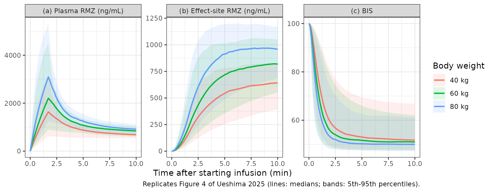
The paper’s Figure 4 medians were digitised by the maintainers. The table compares them with the median of the simulated cohort at the same weight and with the model’s typical-value (no IIV) profile.
fig4_digitised <- tribble(
  ~arm, ~quantity, ~time, ~published,
  "40 kg", "Cc", 1.71, 1652,
  "60 kg", "Cc", 1.71, 2359,
  "80 kg", "Cc", 1.71, 3054,
  "40 kg", "Cc", 3, 1174,
  "60 kg", "Cc", 3, 1522,
  "80 kg", "Cc", 3, 1815,
  "40 kg", "Cc", 5, 859,
  "60 kg", "Cc", 5, 1054,
  "80 kg", "Cc", 5, 1196,
  "40 kg", "Cc", 10, 685,
  "60 kg", "Cc", 10, 804,
  "80 kg", "Cc", 10, 902,
  "40 kg", "effect", 3, 392,
  "60 kg", "effect", 3, 559,
  "80 kg", "effect", 3, 703,
  "40 kg", "effect", 8, 635,
  "60 kg", "effect", 8, 817,
  "80 kg", "effect", 8, 954,
  "60 kg", "BIS", 10, 52
)

as_long <- function(d) {
  d |>
    select(id, arm, time, Cc, effect, BIS) |>
    pivot_longer(c(Cc, effect, BIS), names_to = "quantity", values_to = "value")
}
sim_median <- as_long(sim_fig4) |>
  group_by(arm, quantity, time) |>
  summarise(sim_median = median(value), .groups = "drop")
typ_value <- as_long(sim_typ) |>
  select(arm, quantity, time, typical = value)

fig4_check <- fig4_digitised |>
  left_join(sim_median, by = c("arm", "quantity", "time")) |>
  left_join(typ_value, by = c("arm", "quantity", "time")) |>
  mutate(
    pct_median = 100 * (sim_median - published) / published,
    pct_typical = 100 * (typical - published) / published
  )

stopifnot(
  nrow(fig4_check) == nrow(fig4_digitised),
  !anyNA(fig4_check$sim_median),
  !anyNA(fig4_check$typical)
)

fig4_check |>
  mutate(
    across(c(sim_median, typical), \(x) signif(x, 4)),
    across(c(pct_median, pct_typical), \(x) round(x, 1))
  ) |>
  rename(
    "Weight" = arm,
    "Quantity" = quantity,
    "Time (min)" = time,
    "Figure 4 median (digitised)" = published,
    "Simulated median" = sim_median,
    "Difference, median (%)" = pct_median,
    "Typical value" = typical,
    "Difference, typical (%)" = pct_typical
  ) |>
knitr::kable(caption = "Simulated medians and typical values vs. digitised Figure 4 medians.")| Weight | Quantity | Time (min) | Figure 4 median (digitised) | Simulated median | Typical value | Difference, median (%) | Difference, typical (%) |
|---|---|---|---|---|---|---|---|
| 40 kg | Cc | 1.71 | 1652 | 1637.00 | 1641.00 | -0.9 | -0.7 |
| 60 kg | Cc | 1.71 | 2359 | 2206.00 | 2357.00 | -6.5 | -0.1 |
| 80 kg | Cc | 1.71 | 3054 | 3095.00 | 3023.00 | 1.4 | -1.0 |
| 40 kg | Cc | 3.00 | 1174 | 1191.00 | 1239.00 | 1.5 | 5.5 |
| 60 kg | Cc | 3.00 | 1522 | 1518.00 | 1672.00 | -0.3 | 9.9 |
| 80 kg | Cc | 3.00 | 1815 | 1809.00 | 2026.00 | -0.3 | 11.6 |
| 40 kg | Cc | 5.00 | 859 | 875.30 | 940.30 | 1.9 | 9.5 |
| 60 kg | Cc | 5.00 | 1054 | 1080.00 | 1187.00 | 2.4 | 12.6 |
| 80 kg | Cc | 5.00 | 1196 | 1249.00 | 1357.00 | 4.4 | 13.5 |
| 40 kg | Cc | 10.00 | 685 | 685.40 | 725.50 | 0.1 | 5.9 |
| 60 kg | Cc | 10.00 | 804 | 843.80 | 856.60 | 4.9 | 6.5 |
| 80 kg | Cc | 10.00 | 902 | 915.70 | 937.70 | 1.5 | 4.0 |
| 40 kg | effect | 3.00 | 392 | 383.60 | 386.20 | -2.2 | -1.5 |
| 60 kg | effect | 3.00 | 559 | 520.70 | 547.90 | -6.9 | -2.0 |
| 80 kg | effect | 3.00 | 703 | 709.50 | 695.00 | 0.9 | -1.1 |
| 40 kg | effect | 8.00 | 635 | 619.60 | 642.70 | -2.4 | 1.2 |
| 60 kg | effect | 8.00 | 817 | 801.40 | 838.40 | -1.9 | 2.6 |
| 80 kg | effect | 8.00 | 954 | 965.50 | 992.20 | 1.2 | 4.0 |
| 60 kg | BIS | 10.00 | 52 | 51.02 | 50.62 | -1.9 | -2.6 |
# The typical-value peak is deterministic, so that check is tight: a misread
# clearance, volume, weight exponent or dose unit moves it by tens of
# percent. The simulated medians come from 200 patients per arm, whose median
# carries a Monte Carlo error of several percent at the peak (IIV on V1 is
# 89.9%), so they are gated on their average and with a per-point envelope.
peak <- fig4_check$quantity == "Cc" & fig4_check$time == 1.71
stopifnot(
  all(abs(fig4_check$pct_typical[peak]) < 5),
  mean(abs(fig4_check$pct_median)) < 8,
  all(abs(fig4_check$pct_median) < 20)
)
The simulated medians follow the digitised curves within a few percent at every time and weight. The typical-value curve matches the peak but runs up to 13% above the median plasma concentration during redistribution (3-5 min). With the large IIV on V1, the median of the stochastic profiles falls below the typical-value curve once redistribution dominates, which is why Figure 4 is compared with the simulated median rather than the typical value.
Observed medians (Table 1)
Table 1 reports the median and range of all 60 observed remimazolam
and CNS 7054 concentrations and BIS values, pooled over the 1, 3 and 5
min samples. The study cohort is compared with these after adding
residual error (sim, the simulated observation).
# rxode2 returns the simulated observation (with residual error) for the
# endpoint whose dvid is on the row in `sim`; derive the other two from
# their individual predictions with the model's own log-normal error.
sd_tab <- c(
  Cc = 0.0879,
  Cc_cns7054 = 0.0918,
  BIS = 0.138
)
study_obs <- sim_study |>
  mutate(
    obs_Cc = Cc * exp(rnorm(n(), 0, sd_tab[["Cc"]])),
    obs_cns7054 = Cc_cns7054 * exp(rnorm(n(), 0, sd_tab[["Cc_cns7054"]])),
    obs_BIS = BIS * exp(rnorm(n(), 0, sd_tab[["BIS"]]))
  )

table1 <- tibble(
  quantity = c("Remimazolam (ng/mL)", "CNS 7054 (ng/mL)", "BIS"),
  published_median = c(1159, 485, 53),
  published_range = c("745.4-2471.3", "103-1568.9", "36-83"),
  sim_median = c(
    median(study_obs$obs_Cc),
    median(study_obs$obs_cns7054),
    median(study_obs$obs_BIS)
  ),
  sim_p05 = c(
    quantile(study_obs$obs_Cc, 0.05),
    quantile(study_obs$obs_cns7054, 0.05),
    quantile(study_obs$obs_BIS, 0.05)
  ),
  sim_p95 = c(
    quantile(study_obs$obs_Cc, 0.95),
    quantile(study_obs$obs_cns7054, 0.95),
    quantile(study_obs$obs_BIS, 0.95)
  )
) |>
  mutate(pct_diff = 100 * (sim_median - published_median) / published_median)

table1 |>
  mutate(across(c(sim_median, sim_p05, sim_p95), \(x) signif(x, 3)), pct_diff = round(pct_diff, 1)) |>
  rename(
    "Quantity" = quantity,
    "Table 1 median" = published_median,
    "Table 1 range" = published_range,
    "Simulated median" = sim_median,
    "Simulated 5th pct" = sim_p05,
    "Simulated 95th pct" = sim_p95,
    "Median difference (%)" = pct_diff
  ) |>
knitr::kable(caption = "Pooled 1/3/5-min observations: simulated study cohort vs. Ueshima 2025 Table 1.")| Quantity | Table 1 median | Table 1 range | Simulated median | Simulated 5th pct | Simulated 95th pct | Median difference (%) |
|---|---|---|---|---|---|---|
| Remimazolam (ng/mL) | 1159 | 745.4-2471.3 | 1120.0 | 630.0 | 2140.0 | -3.3 |
| CNS 7054 (ng/mL) | 485 | 103-1568.9 | 524.0 | 89.2 | 1480.0 | 8.0 |
| BIS | 53 | 36-83 | 51.8 | 41.4 | 68.9 | -2.3 |
PKNCA validation
The paper reports no NCA table. PKNCA is run on the simulated Figure 4 cohorts over the 0-10 min window to obtain Cmax, Tmax and AUC0-10 of remimazolam and CNS 7054 per weight. Remimazolam Cmax and Tmax are then compared with the digitised peak of Figure 4a.
dose_df <- events_fig4 |>
  filter(evid == 1L) |>
  select(id, time, amt, arm)
dose_obj <- PKNCA::PKNCAdose(dose_df, amt ~ time | arm + id)

intervals <- data.frame(start = 0, end = 10, cmax = TRUE, tmax = TRUE, auclast = TRUE)

nca_parent_in <- sim_fig4 |>
  filter(!is.na(Cc)) |>
  select(id, time, Cc, arm)
nca_parent <- PKNCA::pk.nca(PKNCA::PKNCAdata(
  PKNCA::PKNCAconc(nca_parent_in, Cc ~ time | arm + id),
  dose_obj,
  intervals = intervals
))

nca_metab_in <- sim_fig4 |>
  filter(!is.na(Cc_cns7054)) |>
  select(id, time, Cc_cns7054, arm)
nca_metab <- PKNCA::pk.nca(PKNCA::PKNCAdata(
  PKNCA::PKNCAconc(nca_metab_in, Cc_cns7054 ~ time | arm + id),
  dose_obj,
  intervals = intervals
))

summary(nca_parent)
#>  start end   arm   N      auclast        cmax              tmax
#>      0  10 40 kg 200  8730 [31.8] 1520 [56.4] 1.71 [1.71, 10.0]
#>      0  10 60 kg 200 11700 [25.4] 2210 [53.6] 1.71 [1.71, 1.71]
#>      0  10 80 kg 200 14000 [22.6] 2910 [50.2] 1.71 [1.71, 10.0]
#>
#> Caption: auclast, cmax: geometric mean and geometric coefficient of variation; tmax: median and range; N: number of subjects
summary(nca_metab)
#>  start end   arm   N     auclast        cmax              tmax
#>      0  10 40 kg 200 3300 [59.2]  730 [53.3] 10.0 [10.0, 10.0]
#>      0  10 60 kg 200 5710 [50.7] 1200 [45.4] 10.0 [10.0, 10.0]
#>      0  10 80 kg 200 8180 [45.8] 1640 [38.1] 10.0 [10.0, 10.0]
#>
#> Caption: auclast, cmax: geometric mean and geometric coefficient of variation; tmax: median and range; N: number of subjects
published_nca <- tribble(
  ~arm, ~cmax, ~tmax,
  "40 kg", 1652, 1.71,
  "60 kg", 2359, 1.71,
  "80 kg", 3054, 1.71
)

cmp <- nlmixr2lib::ncaComparisonTable(
  simulated = nca_parent,
  reference = published_nca,
  by = "arm",
  units = c(cmax = "ng/mL", tmax = "min"),
  tolerance_pct = 20
)

knitr::kable(
  cmp,
  caption = "Remimazolam NCA (median of 200 simulated patients per weight) vs. the digitised Figure 4a peak. * differs by >20%."
)| NCA parameter | arm | Reference | Simulated | % diff |
|---|---|---|---|---|
| Cmax (ng/mL) | 40 kg | 1650 | 1640 | -0.9% |
| Cmax (ng/mL) | 60 kg | 2360 | 2210 | -6.5% |
| Cmax (ng/mL) | 80 kg | 3050 | 3100 | +1.4% |
| Tmax (min) | 40 kg | 1.71 | 1.71 | +0.0% |
| Tmax (min) | 60 kg | 1.71 | 1.71 | +0.0% |
| Tmax (min) | 80 kg | 1.71 | 1.71 | +0.0% |
No row differs by more than 20%. The simulated Tmax is the end of the induction infusion, as in Figure 4a.
Assumptions and deviations
-
IIV percentages read as CVs. Tables 2-4 give the
inter-individual variability as a percentage for the exponential model
of Methods Eq. 2, without stating whether it is a CV or the square root
of the variance x
- The percentages were converted with
omega^2 = log(CV^2 + 1). The confidence intervals are symmetric on the percentage scale and so cannot separate the two readings. The reading matters for the wide rows: under the square-root reading the variances of V1, CLM, V1M and EC50 would be 0.808, 0.445, 0.332 and 0.972 instead of 0.592, 0.368, 0.287 and 0.679. Figure 4 does not settle it either: with 1000 simulated patients per weight, both readings reproduce the digitised plasma and effect-site medians within about 2-3% on average (the CV reading fits the effect-site curve slightly better, 1.2% vs 3.4% mean absolute difference), which is within the Monte Carlo and digitising error.
- The percentages were converted with
- EC50 IIV taken from Table 4 (98.6%), not the Results text (35.1%). The Results paragraph says “The inter-individual variability for EC50 was 35.1%”, while Table 4 prints 98.6% with a 95% CI of 29.8-167%, an RSE of 35.6% and a bootstrap median of 98.0%. The table value is internally consistent (98.6 +/- 1.96 x 0.356 x 98.6 reproduces the printed interval), the bootstrap agrees, and every other variability in the Results text matches its table, so the text value was treated as a typographical error.
-
Weight on CNS 7054 V2M and Q2M is linear per 75 kg.
Methods say that body weight was included allometrically on all
disposition parameters with exponents 0.75 for clearance and 1 for
volume. The final-model row equations in Tables 2 and 3, however, apply
weight only to CL (
(BW/60.4)^0.75) and to the literature-fixed V2M and Q2M as(BW/75)with units of “L/75 kg” and “L/min/75 kg”. The printed equations were followed, so Q2M scales with exponent 1 and V1, V2, V3, Q2, Q3, CLM and V1M are not weight-scaled. - Doses are remimazolam base. Anerem is labelled and dosed as remimazolam, and the simulated peak at loss of consciousness reproduces Figure 4a within 2% without a salt correction (a besylate-to-base factor would lower it by about 26%).
- No molecular-weight conversion between parent and metabolite. The paper does not state one, so remimazolam clearance enters the transit compartment 1:1 by mass, and the CNS 7054 volumes and clearance are apparent values on that basis.
- Fixed literature values. kT, V3, V2M, Q2, Q3 and Q2M are the values printed in Tables 2 and 3 (from Schuttler 2020), and kE0 = 0.135 1/min is the value printed in Table 4 (from Zhou 2020). They were not re-derived from those papers.
-
Residual error. The exponential residual error of
Methods Eq. 1 (
C = C_pred x exp(epsilon)) is encoded aslnorm()with the tabulated percentage as the log-scale SD, for remimazolam, CNS 7054 and BIS. - Sequential fit encoded jointly. The authors fitted the PD on each patient’s Bayesian PK estimates. The packaged model links the PK and PD directly, which is equivalent for simulation.
- Virtual-cohort covariates. The individual weights and loss-of-consciousness times are not published. The study cohort draws weight from a normal distribution (mean 60.4 kg, SD 8 kg) and the loss-of-consciousness time from a log-normal distribution (median 1.71 min, log-SD 0.25), each truncated to the Table 1 range.
- Errata. Crossref registered no correction or update for the article as of 2026-11-05.