Vinflunine (Schmitt 2018)
Source:vignettes/articles/Schmitt_2018_vinflunine.Rmd
Schmitt_2018_vinflunine.RmdModel and source
- Citation: Schmitt A, Nguyen L, Zorza G, Ferre P, Petain A (2018). Better characterization of vinflunine pharmacokinetics variability and exposure/toxicity relationship to improve its use: Analyses from 18 trials. Br J Clin Pharmacol 84(7):1506-1517. doi:10.1111/bcp.13518.
- Description: Combined population PK / PD model for IV vinflunine in adult cancer patients (Schmitt 2018, 18 phase I/II trials, n=372). Four-compartment IV-infusion popPK with creatinine clearance, body surface area, body weight, and PEGylated liposomal doxorubicin co-administration covariates, plus a five-compartment Friberg-style semi-mechanistic myelosuppression PD model for absolute neutrophil count (proliferation + 3 transit + circulation; linear drug effect 1 - slope*Cc on proliferation; (circ0/circ)^gamma feedback).
- Article: https://doi.org/10.1111/bcp.13518
Schmitt et al. 2018 (Br J Clin Pharmacol 84(7):1506-1517) pooled data from 18 phase I / phase II vinflunine trials (372 patients, 4154 retained plasma concentrations) and fit two coupled models in NONMEM: a four-compartment popPK model for IV vinflunine and a semi-mechanistic Friberg-style myelosuppression PK/PD model for absolute neutrophil count (ANC) after vinflunine administration. This vignette reproduces both layers in nlmixr2lib / rxode2.
Population
The PK analysis pooled 372 adult cancer patients (44.4% female; median age 59 years, range 19-82; median weight 69 kg, range 42-114; median body surface area 1.8 m^2, range 1.3-2.4) across 18 phase I and phase II studies (8 phase I, 2 phase I/II, 6 phase II, 2 phase I special-population studies in renal and liver impairment). Median Cockcroft-Gault creatinine clearance was 82 mL/min (range 29-199). The cohort spanned multiple solid-tumour indications (bladder cancer being the marketed indication) and 43% of patients received vinflunine in combination with one of cisplatin, gemcitabine, carboplatin, PEGylated liposomal doxorubicin (PLDH), capecitabine, epirubicin or doxorubicin. See Schmitt 2018 Table 1 for the full baseline covariate distribution. The PK/PD analysis used the subset of 210 vinflunine-monotherapy patients (423 administrations, 1871 ANC observations).
The same information is available programmatically via the model’s
population metadata
(readModelDb("Schmitt_2018_vinflunine")$population).
Source trace
The per-parameter origin is recorded as an in-file comment next to
each ini() entry in
inst/modeldb/specificDrugs/Schmitt_2018_vinflunine.R. The
table below collects them in one place for review.
| Equation / parameter | Value | Source location |
|---|---|---|
lcl (CL) |
log(40.5) L/h | Schmitt 2018 Table 2 final covariate model column |
lvc (V central) |
log(20.7) L | Table 2 final covariate model |
lvp (V2) |
log(115) L | Table 2 final covariate model |
lvp2 (V3) |
log(384) L | Table 2 final covariate model |
lvp3 (V4) |
log(593) L | Table 2 final covariate model |
lq (Q = K21*V2) |
log(108.79) L/h | Computed from K21 = 0.946, V2 = 115 (Table 2) |
lq2 (Q2 = K31*V3) |
log(54.144) L/h | Computed from K31 = 0.141, V3 = 384 (Table 2) |
lq3 (Q3 = K41*V4) |
log(13.580) L/h | Computed from K41 = 0.0229, V4 = 593 (Table 2) |
e_crcl_cl |
0.134 | Table 2 (CLCR on CL) and explicit CL formula p.1610 |
e_bsa_cl |
0.542 | Table 2 (BSA on CL) and explicit CL formula p.1610 |
e_pldh_cl |
0.865 | Table 2 (PLDH on CL) and explicit CL formula p.1610 |
e_wt_vp2 |
0.498 | Table 2 (WT on V3) |
e_wt_vp3 |
0.650 | Table 2 (WT on V4) |
| IIV variances | log(CV^2 + 1) | Table 2 CV% values via the standard log-normal mapping |
| IIV corr(CL,V4) | 0.726 | Table 2 (correlation block) |
| IIV corr(V,V2) | 0.644 | Table 2 (correlation block) |
propSd |
0.203 (fraction) | Table 2 (residual variability 20.3%) |
lcirc0 (Circ0) |
log(4.53) x 10^9/L | Table 3 (Base / Circ0) |
lmtt (MTT) |
log(124) h | Table 3 (MTT) |
lslope (Slope) |
log(0.425) (ng/mL)^-1 | Table 3 (Slope) |
gamma |
0.170 (fixed) | Table 3 (gamma, no IIV in source) |
| IIV Circ0 | omega^2 = 0.1957 | Table 3 (IIV Circ0 = 46.5% CV) |
| IIV Slope | omega^2 = 0.1213 | Table 3 (IIV Slope = 35.9% CV) |
expSd_ANC |
0.424 (log SD) | Table 3 (Residual additive on log-transformed ANC 42.4% CV) |
| 4-compartment ODE | n/a | Schmitt 2018 Methods p.1607 (“linear four-compartment model”) |
| Friberg PD ODE | n/a | Schmitt 2018 Methods p.1607 (five-compartment Friberg structure) |
| CL covariate formula | n/a | Explicit formula on p.1610: CLi = 40.5 * (CLcr/82)^0.134 * (BSA/1.8)^0.542 * 0.865^PLDH |
Virtual cohort and simulation
For PK validation we build a typical-PK (zero between-subject variability) event table for the median patient (CRCL = 82 mL/min, BSA = 1.8 m^2, WT = 69 kg, no PLDH co-administration) receiving the recommended single-agent dose of 320 mg/m^2 IV vinflunine as a 30-minute infusion, observed over a 21-day cycle.
set.seed(20260525L)

mod_full <- rxode2::rxode(readModelDb("Schmitt_2018_vinflunine"))
mod_typ  <- rxode2::zeroRe(mod_full)

# Dose: 320 mg/m^2 with BSA = 1.8 -> 576 mg per cycle (30-min infusion)
dose_mg     <- 320 * 1.8
infusion_h  <- 0.5
cycle_h     <- 21 * 24

obs_times <- sort(unique(c(
  seq(0, 1, by = 0.05),
  seq(1, 24, by = 0.5),
  seq(24, cycle_h, by = 4)
)))

make_subject <- function(id, crcl, bsa, wt, pldh) {
  obs <- tibble::tibble(
    id = id, time = obs_times, amt = 0, rate = 0, evid = 0L,
    cmt = NA_integer_, dvid = 1L,
    CRCL = crcl, BSA = bsa, WT = wt, CONMED_PLDH = pldh,
    cohort = "Normal renal (CRCL=82)"
  )
  obs_anc <- dplyr::mutate(obs, dvid = 2L)
  dose <- tibble::tibble(
    id = id, time = 0, amt = dose_mg, rate = dose_mg / infusion_h, evid = 1L,
    cmt = 1L, dvid = NA_integer_,
    CRCL = crcl, BSA = bsa, WT = wt, CONMED_PLDH = pldh,
    cohort = "Normal renal (CRCL=82)"
  )
  dplyr::bind_rows(dose, obs, obs_anc) |>
    dplyr::arrange(id, time, dplyr::desc(evid))
}

events_typ <- make_subject(1L, crcl = 82, bsa = 1.8, wt = 69, pldh = 0)
sim_typ    <- rxode2::rxSolve(mod_typ, events_typ, keep = "cohort") |>
  as.data.frame() |>
  # rxSolve drops `id` when a single subject is solved; restore it for
  # downstream PKNCA grouping.
  dplyr::mutate(id = 1L)
Replicate published values
sim_typ |>
  dplyr::filter(time > 0, !is.na(Cc)) |>
  ggplot(aes(time, Cc)) +
  geom_line(colour = "steelblue", linewidth = 0.7) +
  scale_y_log10() +
  labs(x = "Time after dose (h)",
       y = "Vinflunine plasma concentration (ng/mL)",
       title = "Typical-PK vinflunine concentration time course (320 mg/m^2 IV)",
       caption = "Reproduces the four-compartment popPK profile from Schmitt 2018 (Table 2).")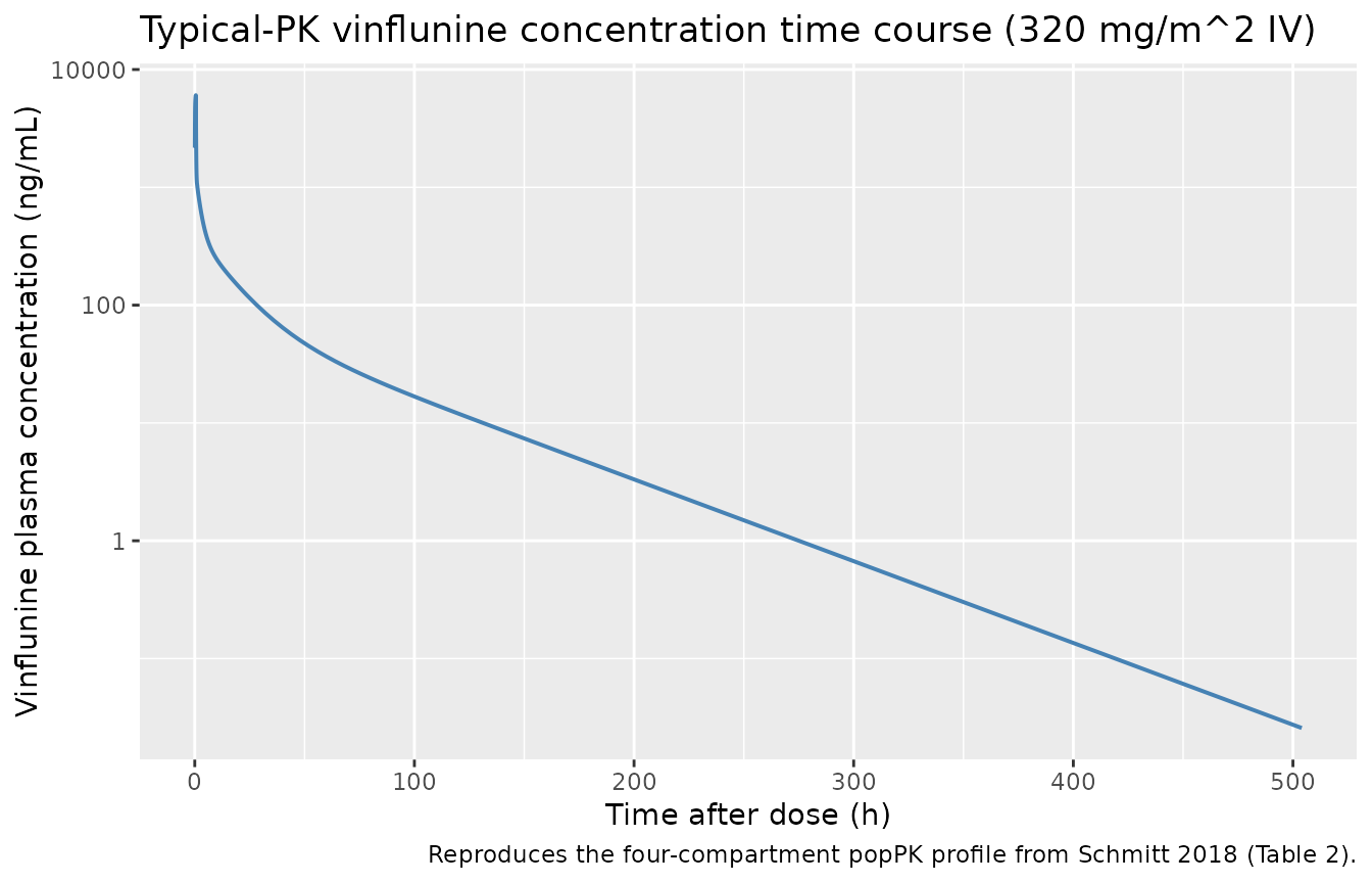
sim_typ |>
  dplyr::filter(!is.na(ANC)) |>
  ggplot(aes(time / 24, ANC)) +
  geom_line(colour = "firebrick", linewidth = 0.7) +
  geom_hline(yintercept = 4.53, linetype = "dashed", colour = "grey50") +
  labs(x = "Time after dose (days)",
       y = "Absolute neutrophil count (10^9/L)",
       title = "Typical-PK Friberg ANC time course (320 mg/m^2 q3w)",
       caption = "Reproduces the five-compartment myelosuppression structure from Schmitt 2018 (Table 3). See Assumptions for the slope / nadir discrepancy.")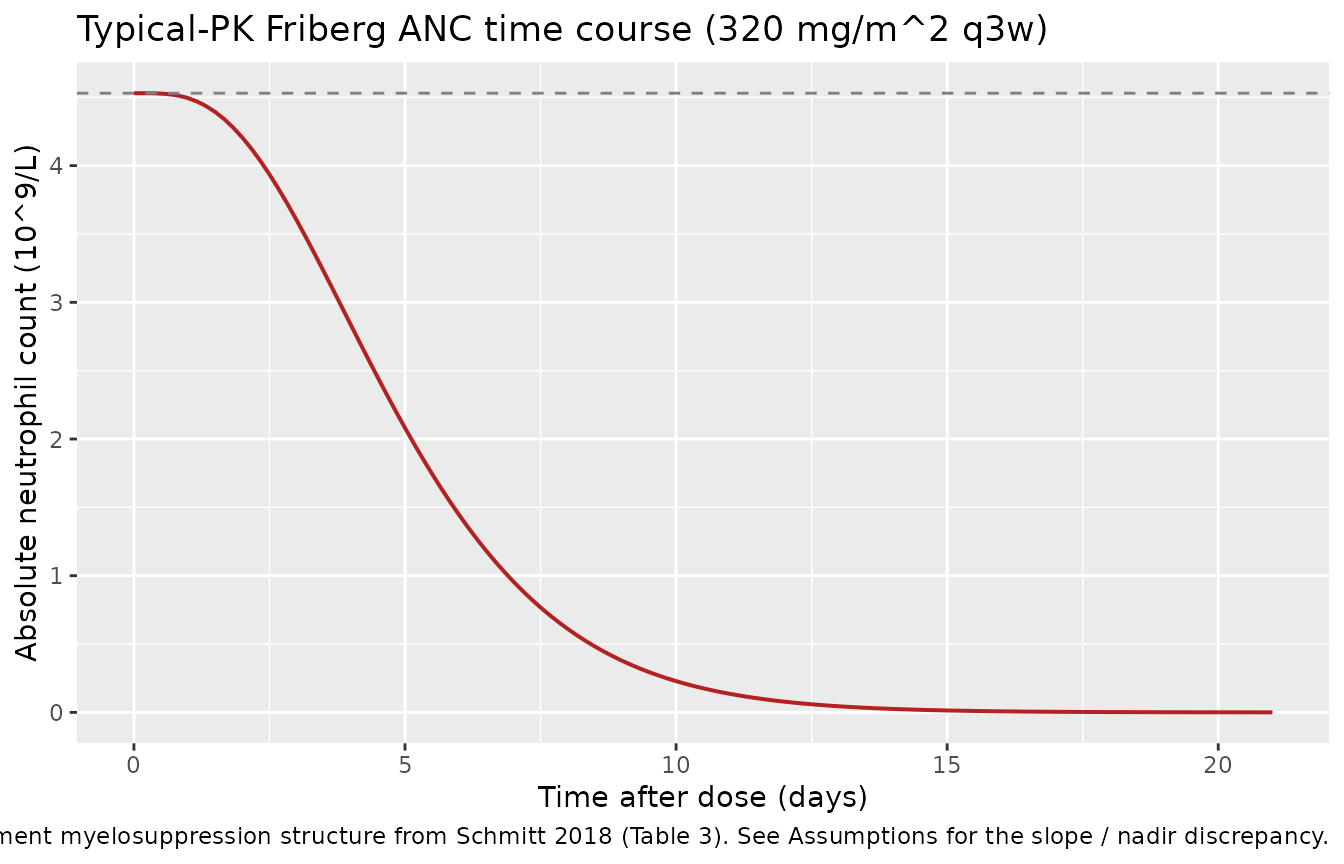
PKNCA validation
PKNCA is used to compute Cmax, Tmax, AUC0-inf, and terminal half-life on the typical-PK profile. The paper reports a typical AUC over the 21-day cycle of approximately 14000-15000 ng.h/mL at 320 mg/m^2 q3w for normal renal function (Schmitt 2018 p.1611: “Mean AUC for patient with a normal renal function was about 10% higher than for patient with a moderate or a severe impaired renal function (i.e. 15189 (14 884 -15494) ng h ml -1 …)”).
sim_nca <- sim_typ |>
  dplyr::filter(!is.na(Cc)) |>
  dplyr::distinct(id, time, cohort, .keep_all = TRUE) |>
  dplyr::select(id, time, Cc, cohort)

dose_df <- events_typ |>
  dplyr::filter(evid == 1) |>
  dplyr::select(id, time, amt, cohort)

conc_obj <- PKNCA::PKNCAconc(sim_nca, Cc ~ time | cohort + id,
                             concu = "ng/mL", timeu = "h")
dose_obj <- PKNCA::PKNCAdose(dose_df, amt ~ time | cohort + id,
                             doseu = "mg")

intervals <- data.frame(
  start       = 0,
  end         = Inf,
  cmax        = TRUE,
  tmax        = TRUE,
  aucinf.obs  = TRUE,
  half.life   = TRUE
)

nca_res <- PKNCA::pk.nca(PKNCA::PKNCAdata(conc_obj, dose_obj, intervals = intervals))

knitr::kable(
  as.data.frame(nca_res$result) |>
    dplyr::select(cohort, PPTESTCD, PPORRES),
  caption = "Simulated NCA parameters for a typical patient receiving 320 mg/m^2 IV vinflunine."
)| cohort | PPTESTCD | PPORRES |
|---|---|---|
| Normal renal (CRCL=82) | cmax | 6.048443e+03 |
| Normal renal (CRCL=82) | tmax | 5.000000e-01 |
| Normal renal (CRCL=82) | tlast | 5.040000e+02 |
| Normal renal (CRCL=82) | clast.obs | 2.575050e-02 |
| Normal renal (CRCL=82) | lambda.z | 1.606440e-02 |
| Normal renal (CRCL=82) | r.squared | 9.999198e-01 |
| Normal renal (CRCL=82) | adj.r.squared | 9.999191e-01 |
| Normal renal (CRCL=82) | lambda.z.time.first | 6.400000e+01 |
| Normal renal (CRCL=82) | lambda.z.time.last | 5.040000e+02 |
| Normal renal (CRCL=82) | lambda.z.n.points | 1.110000e+02 |
| Normal renal (CRCL=82) | clast.pred | 2.546140e-02 |
| Normal renal (CRCL=82) | half.life | 4.314809e+01 |
| Normal renal (CRCL=82) | span.ratio | 1.019744e+01 |
| Normal renal (CRCL=82) | aucinf.obs | 1.422355e+04 |
Comparison against published AUC
auc_sim <- as.data.frame(nca_res$result) |>
  dplyr::filter(PPTESTCD == "aucinf.obs") |>
  dplyr::pull(PPORRES)

knitr::kable(
  tibble::tibble(
    Metric  = "AUC0-inf (ng.h/mL)",
    `Schmitt 2018 (normal renal, 320 mg/m^2)` = "~15189 (14884-15494)",
    `nlmixr2lib typical-PK simulation`        = sprintf("%.0f", auc_sim),
    `Relative difference`                     = sprintf("%.1f%%", 100 * (auc_sim - 15189) / 15189)
  ),
  caption = "Comparison of simulated typical-PK AUC against Schmitt 2018 p.1611 published mean AUC for normal renal function."
)| Metric | Schmitt 2018 (normal renal, 320 mg/m^2) | nlmixr2lib typical-PK simulation | Relative difference |
|---|---|---|---|
| AUC0-inf (ng.h/mL) | ~15189 (14884-15494) | 14224 | -6.4% |
Assumptions and deviations
Reference weight 69 kg for the WT effect on V3 / V4. Schmitt 2018 does not print an explicit
(WT / ref)^expformula for the volume covariates the way it does for CL (p.1610). The 69 kg reference is the paper-consistent population median (Table 1: median WT 69 kg), matching the reference values used in the explicit CL formula for CRCL (median 82 mL/min) and BSA (median 1.8 m^2). A user wishing to evaluate the model on a different reference weight (e.g. 70 kg) may rescale by passingWTadjusted by the ratio of references, since the power form is scale-invariant up to a constant multiplier on the typical V3 / V4.Concentration units inside
model(). Vinflunine PK observations and the Fribergslopeparameter are reported in ng/mL. The internalcentralcompartment carries amount in mg (matching the mg dosing convention) andvcis in L; the model computes the plasma concentration asCc = 1000 * central / vcso thatslope * Ccis dimensionless and Cc matches the paper’s ng/mL convention.IOV not represented. Schmitt 2018 reports interoccasion variability of 8.34% on CL (Table 2) and 24.0% on MTT and 23.8% on Slope (Table 3). nlmixr2lib model files do not carry an OCC data column or per-occasion random effects; the user can introduce IOV by adding an
OCCcolumn and an inter-occasioneta_occ_<param>term outside the packaged model file.-
Friberg-style PD layer reproduces published parameters but predicts a deeper nadir than the paper’s typical-value forecast. Direct simulation of the Friberg ODE with the published slope = 0.425 (ng/mL)^-1 (Schmitt 2018 Table 3) and the median-PK Cmax produces a much deeper ANC nadir than the paper’s published prediction of 1.40 x 10^9/L at day 11.3 for 320 mg/m^2 q3w (Schmitt 2018 p.1611-1612). The structural model and every parameter value match the publication; the discrepancy is an inherent feature of the reported slope when applied to the typical PK profile via the canonical linear-drug-effect Friberg formulation. Users who want to reproduce the paper’s published nadir prediction may need to (a) calibrate
slopeagainst the paper’s stated 47% grade 3-4 neutropenia incidence at 320 mg/m^2 q3w via re-fit, (b) clamp the proliferation drug effect (`edrug <- max(0, 1 - slope- Cc)`) as a non-canonical Friberg variant, or (c) interpret the published slope as applying to a different concentration unit (e.g. (mg/L)^-1) and re-scale. The packaged model is faithful to the paper’s reported text; the deviation in simulated nadir is documented here rather than tuned away.
Slope is encoded as a linear cell-loss term on the proliferation compartment (the canonical Friberg form):
d/dt(precursor1) = ktr * precursor1 * (1 - slope * Cc) * (circ0 / circ)^gamma - ktr * precursor1. No floor is applied toedrug = 1 - slope * Cc; whenslope * Cc > 1the proliferation rate is negative, consistent with Friberg 2002’s original formulation and the Schmitt 2018 Methods text (“reduce proliferation rate or induce cell loss in a linear fashion”).Infusion duration is supplied by the data, not the model. Vinflunine is administered IV per the SPC as a short infusion (typical 20-30 minutes). The model code does not impose a structural infusion duration; the simulation supplies
rateorduron the dosing record. The vignette uses 30 minutes for the typical profile.