Trastuzumab + doxorubicin cardiotoxicity (Yu 2025)
Source:vignettes/articles/Yu_2025_trastuzumab_doxorubicin_cardiotoxicity.Rmd
Yu_2025_trastuzumab_doxorubicin_cardiotoxicity.RmdModel and source
Yu 2025 extends an earlier quantitative systems toxicology (QST) model of doxorubicin (DOX) cardiotoxicity in AC16 human cardiomyocytes to trastuzumab (TmAb) and to the DOX + TmAb combination, and then scales the BNP-release layer to patients. The paper fits three in vitro layers and one clinical layer. They are packaged as three models:
-
Yu_2025_doxorubicin_trastuzumab_ac16: the apoptosis protein-dynamics layer (caspase-9 and caspase-3) and the cardiomyocyte-death layer (AC16 relative viability). The paper fits these two layers one after the other, holding the protein-dynamics estimates fixed while fitting the death layer. The death layer is driven by the protein layer’s caspase-3 state, so the two layers form one coupled ODE system. -
Yu_2025_doxorubicin_trastuzumab_bnp_ac16: the in vitro BNP-release (cardiomyocyte-injury biomarker) layer, which is independent of the caspase layers. -
Yu_2025_doxorubicin_trastuzumab_bnp_human: the clinical scale-up of the BNP layer, driven by an externally supplied trastuzumab concentration in cardiac interstitial fluid.
mod_ac16 <- readModelDb("Yu_2025_doxorubicin_trastuzumab_ac16")
mod_bnp <- readModelDb("Yu_2025_doxorubicin_trastuzumab_bnp_ac16")
mod_hum <- readModelDb("Yu_2025_doxorubicin_trastuzumab_bnp_human")- Citation: Yu S, Mody H, Vaidya TR, Kagan L, Ait-Oudhia S. Mitigating Trastuzumab-Doxorubicin Cardiotoxicity With Multiscale Quantitative Systems Toxicology and PBPK-Toxicodynamic Predictive Modeling Framework. CPT Pharmacometrics Syst Pharmacol. 2025;14(10):1625-1636. doi:10.1002/psp4.70087
- Article: https://doi.org/10.1002/psp4.70087
Population
In vitro. AC16 cells (immortalised, HER2-positive human cardiomyocytes, MilliporeSigma) were cultured in DMEM with 10% FBS at 37 C and 5% CO2. Each “individual” in the Monolix fit is a treatment group, so the random effects are inter-treatment-group variability, not inter-individual variability. The paper ran three experiments:
- Caspase-9 and caspase-3 activity (MILLIPLEX / Luminex) at 0, 3, 6, 12, 24, 48 and 72 h after control, DOX 100 nM, TmAb 25 uM, or DOX 50 nM + TmAb 12.5 uM (Figure 2).
- Cell viability (CCK-8) over 96 h after DOX 1.1, 10.5 or 25 nM, TmAb 13.3, 23 or 28.4 uM, all nine DOX x TmAb combinations, and control (Figure 3).
- BNP in the culture supernatant (ELISA) over 72 h after DOX 25 nM, TmAb 23 uM, their combination, and control (Figure 4).
Clinical. The BNP scale-up used mean NT-proBNP from 11 breast cancer patients treated with trastuzumab for two cycles: 8 mg/kg over 90 min, then 6 mg/kg three weeks later. The values were digitised from Advani 2017, converted to BNP with the linear relationship of Taki 2018, and normalised to baseline (Figure 5). An external qualification used mean LVEF from 163 HER2-positive early breast cancer patients given 12 months of adjuvant trastuzumab (Jacquinot 2018); LVEF was converted to relative BNP through an NT-proBNP-LVEF regression (Figure 6).
The same information is available programmatically via
rxode2::rxode(mod_ac16)$population (and likewise for the
two BNP models).
Source trace
Every ini() value carries an in-file comment pointing to
its source. The deposited Monolix code is in Supplement Data S1 and S2.
The two supplement files carry the same code.
| Model element | Value | Source location |
|---|---|---|
lkdeg_dox (DOX degradation in medium) |
log(0.022) 1/h, fixed | Table 1 k deg (fix, from Vaidya 2021); Supplement
Kdeg = 0.022
|
c1 |
1.68 | Table 1 |
lsc1 |
log(0.046e-2) nM^-c1 | Table 1 Sc1 (10^-2 nM^-1) 0.046 |
lkcas9s |
log(0.093e-3) 1/h | Table 1 k cas9s (10^-3 h^-1) 0.093 |
lsc2 |
log(0.057) nM^-c2 | Table 1 Sc2
|
lkcas9 |
log(0.083) 1/h | Table 1 |
lkcas3 |
log(0.87) 1/h | Table 1 |
c2 |
0.99 | Table 1 |
c3 |
4.48 | Table 1 |
etalsc1, etalsc2
|
0.049^2, 0.99^2 | Table 1 IIVSc1, IIVSc2 (omega as SD) |
propSd_cas92, propSd_cas33
|
0.18, 0.43 | Table 1 protein-model Ba, Bb
|
lsmax_cas3 |
log(0.23) 1/h | Table 1 Smaxcas3
|
c4 |
1.5 | Table 1 |
lsc50_cas3 |
log(2.56) | Table 1 SC50cas3
|
lktr_death |
log(0.023) 1/h | Table 1 k tr
|
lkgrow |
log(0.035) 1/h | Table 1 k g
|
lkd2 |
log(0.022) 1/nM | Table 1 kd2
|
etalkd2 |
0.69^2 | Table 1 IIVkd2
|
propSd_viability |
0.36 | Table 1 death-model Ba
|
lks |
log(1) 1/h | Table 1 k s
|
lkbnp |
log(0.202) 1/h, fixed | Table 1 k bnp 0.20 (fix); Supplement
Kbnp = 0.202
|
lsbnp1, lsbnp2
|
log(0.086), log(0.005) 1/nM | Table 1 (fixed in the human model) |
propSd_bnp3 (in vitro) |
0.44 | Table 1 BNP-model B
|
lfsct |
log(0.86) | Table 1 f Sct
|
propSd_bnp3 (human) |
0.63 | Table 1 human-model B
|
| DOX degradation ODE | – | Eq 1; Supplement ddt_Cdox
|
Caspase-9 ODEs (cas9s, cas91,
cas92) |
– | Eqs 2-4; Supplement protein-dynamics code |
Caspase-3 transit chain (cas31-cas33) |
– | Eqs 5-7 as coded in the Supplement (see Assumptions) |
Death signal kd1 and transit tr1,
tr2
|
– | Eqs 8-10; Supplement cardiomyocyte-death code |
| Viability ODE | – | Eq 11; Supplement ddt_R
|
| In vitro BNP ODEs | – | Eqs 12-15; Supplement in vitro BNP code |
| Human BNP ODEs | – | Supplement human BNP code (Eqs 13-15 with fSct on the
TmAb slope) |
In vitro caspase signalling (Figure 2)
The typical-value model is solved for the four treatment groups of
the caspase experiment. DOX is applied as a bolus of the medium
concentration (nM) into conc_dox at t = 0. The TmAb
concentration is the time-constant covariate
CONC_TRASTUZUMAB_NM (nM). Observation rows sit on the ODE
state cas92; rxode2 returns every state at those times.
# One treatment group as an event table: DOX bolus (nM) into the medium and
# observations on a named ODE state. CONC_TRASTUZUMAB_NM is constant.
make_group <- function(dox_nm, tmab_nm, times, obs_cmt, id = 1L, dose_cmt = "conc_dox") {
  obs <- data.frame(
    id = id, time = times, evid = 0L, amt = 0, cmt = obs_cmt,
    CONC_TRASTUZUMAB_NM = tmab_nm
  )
  if (dox_nm > 0) {
    dose <- data.frame(
      id = id, time = 0, evid = 1L, amt = dox_nm, cmt = dose_cmt,
      CONC_TRASTUZUMAB_NM = tmab_nm
    )
    obs <- dplyr::bind_rows(dose, obs)
  }
  obs
}

typ_ac16 <- rxode2::zeroRe(rxode2::rxode(mod_ac16))
#> ℹ parameter labels from comments will be replaced by 'label()'
# The BNP models have no random effects, so zeroRe() only zeroes their
# residual error and warns that there is no omega to zero.
typ_bnp <- suppressWarnings(rxode2::zeroRe(rxode2::rxode(mod_bnp)))
typ_hum <- suppressWarnings(rxode2::zeroRe(rxode2::rxode(mod_hum)))
casp_groups <- data.frame(
  group = c("Control", "DOX 100 nM", "TmAb 25 uM", "DOX 50 nM + TmAb 12.5 uM"),
  dox = c(0, 100, 0, 50),
  tmab = c(0, 0, 25000, 12500)
)
sim_casp <- purrr::map_dfr(seq_len(nrow(casp_groups)), function(i) {
  ev <- make_group(casp_groups$dox[i], casp_groups$tmab[i], seq(0, 72, by = 0.5), "cas92")
  as.data.frame(rxode2::rxSolve(typ_ac16, ev)) |>
    dplyr::mutate(group = casp_groups$group[i])
})
#> ℹ omega/sigma items treated as zero: 'etalsc1', 'etalsc2', 'etalkd2'
#> ℹ omega/sigma items treated as zero: 'etalsc1', 'etalsc2', 'etalkd2'
#> ℹ omega/sigma items treated as zero: 'etalsc1', 'etalsc2', 'etalkd2'
#> ℹ omega/sigma items treated as zero: 'etalsc1', 'etalsc2', 'etalkd2'
sim_casp$group <- factor(sim_casp$group, levels = casp_groups$group)

sim_casp |>
  dplyr::select(time, group, `Caspase-9` = cas92, `Caspase-3` = cas33) |>
  tidyr::pivot_longer(c(`Caspase-9`, `Caspase-3`), names_to = "protein", values_to = "rel") |>
  ggplot(aes(time, rel, colour = group)) +
  geom_line(linewidth = 0.9) +
  facet_wrap(~protein, scales = "free_y") +
  labs(x = "Time (h)", y = "Relative protein expression", colour = NULL) +
  theme_bw() +
  theme(legend.position = "bottom")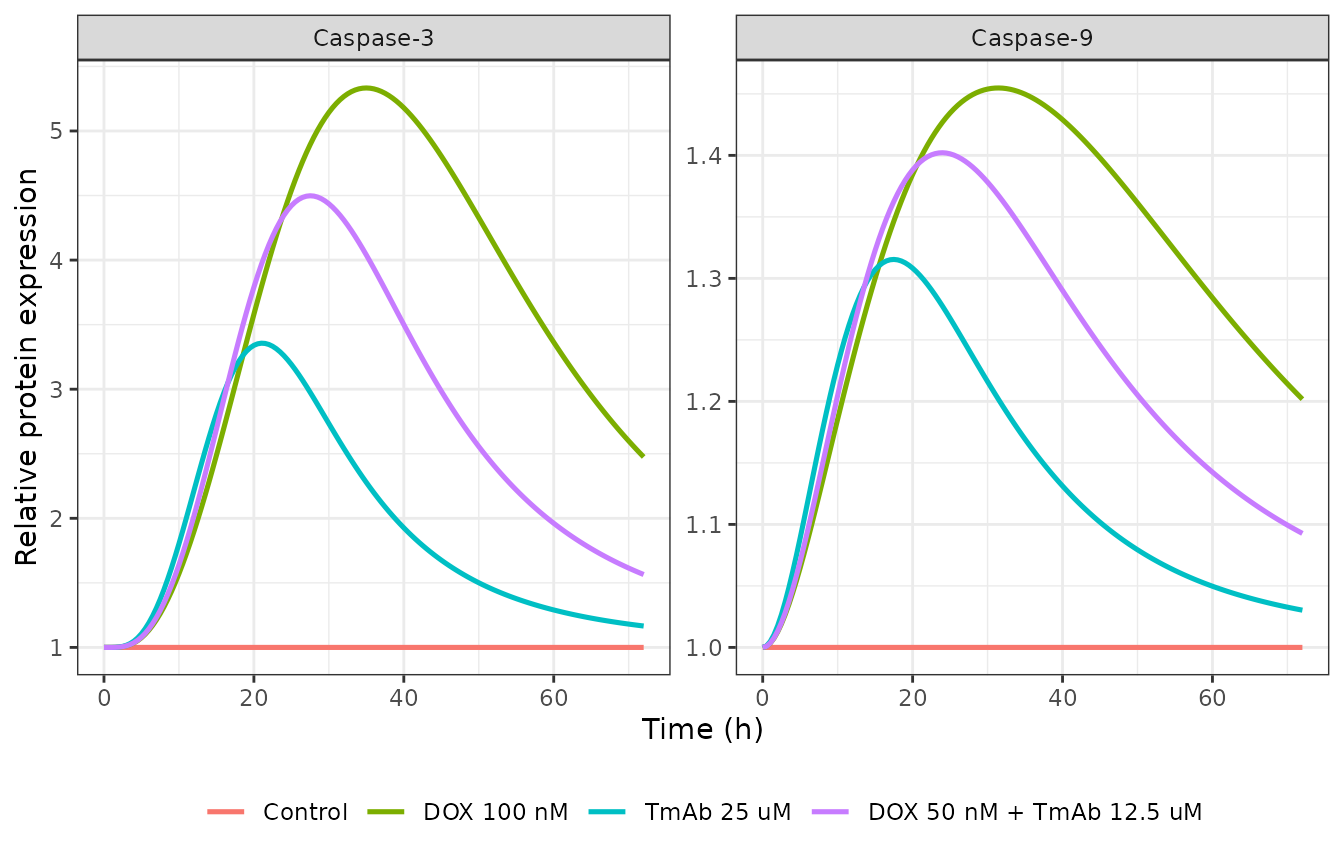
Replicates Figure 2 of Yu 2025: typical-value relative caspase-9 (cas92) and caspase-3 (cas33) activity in AC16 cells over 72 h.
The DOX-only group has no TmAb, and its DOX slope carries only 5% CV between groups. Its typical curve should therefore sit on the published fit. The fit peaks near 1.45 at about 30 h for caspase-9 and near 5.4 at about 35 h for caspase-3 (Figure 2, read from the plot):
casp_peaks <- sim_casp |>
  dplyr::group_by(group) |>
  dplyr::summarise(
    cas92_peak = max(cas92), cas92_tpeak = time[which.max(cas92)],
    cas33_peak = max(cas33), cas33_tpeak = time[which.max(cas33)],
    .groups = "drop"
  )
casp_peaks |>
  dplyr::rename(
    "Group" = group, "Caspase-9 peak" = cas92_peak, "Caspase-9 peak time (h)" = cas92_tpeak,
    "Caspase-3 peak" = cas33_peak, "Caspase-3 peak time (h)" = cas33_tpeak
  ) |>
knitr::kable(digits = 2, caption = "Typical-value caspase peaks per treatment group.")| Group | Caspase-9 peak | Caspase-9 peak time (h) | Caspase-3 peak | Caspase-3 peak time (h) |
|---|---|---|---|---|
| Control | 1.00 | 0.0 | 1.00 | 0.0 |
| DOX 100 nM | 1.45 | 31.5 | 5.33 | 35.0 |
| TmAb 25 uM | 1.32 | 17.5 | 3.36 | 21.0 |
| DOX 50 nM + TmAb 12.5 uM | 1.40 | 24.0 | 4.50 | 27.5 |
dox_pk <- casp_peaks[casp_peaks$group == "DOX 100 nM", ]
ctl_pk <- casp_peaks[casp_peaks$group == "Control", ]
stopifnot(
  # Control: no drug, every state stays at its baseline of 1.
  abs(ctl_pk$cas92_peak - 1) < 1e-6,
  abs(ctl_pk$cas33_peak - 1) < 1e-6,
  # DOX 100 nM against the published fit (digitised peak 1.45 / 5.4).
  abs(dox_pk$cas92_peak / 1.45 - 1) < 0.10,
  abs(dox_pk$cas33_peak / 5.4 - 1) < 0.15
)
The TmAb-containing groups differ more from the published curves,
because the figure shows each group’s individual (empirical-Bayes) fit
and the TmAb slope Sc2 carries a between-group omega of
0.99 (129% CV). The typical TmAb-only caspase-3 curve peaks near 3.4 at
about 21 h, while the published individual fit peaks near 4.2 at about
17 h.
Between-group variability
The spread that the between-group random effects produce is shown below for 100 virtual treatment groups at each of the two single-agent conditions:
rxode2::rxSetSeed(20251)
n_grp <- 100L
ev_vpc <- dplyr::bind_rows(
  purrr::map_dfr(seq_len(n_grp), function(i) {
    make_group(100, 0, seq(0, 72, by = 1), "cas92", id = i) |> dplyr::mutate(cond = "DOX 100 nM")
  }),
  purrr::map_dfr(seq_len(n_grp), function(i) {
    make_group(0, 25000, seq(0, 72, by = 1), "cas92", id = n_grp + i) |> dplyr::mutate(cond = "TmAb 25 uM")
  })
)
stopifnot(!anyDuplicated(ev_vpc[ev_vpc$evid == 0, c("id", "time")]))
sim_vpc <- as.data.frame(rxode2::rxSolve(
  rxode2::rxode(mod_ac16), ev_vpc,
  keep = "cond", returnType = "data.frame"
))
#> ℹ parameter labels from comments will be replaced by 'label()'
vpc_sum <- sim_vpc |>
  dplyr::group_by(cond, time) |>
  dplyr::summarise(
    med = stats::median(cas33),
    lo = stats::quantile(cas33, 0.05), hi = stats::quantile(cas33, 0.95),
    .groups = "drop"
  )
ggplot(vpc_sum, aes(time, med)) +
  geom_ribbon(aes(ymin = lo, ymax = hi), alpha = 0.25, fill = "steelblue") +
  geom_line(linewidth = 0.9, colour = "steelblue4") +
  facet_wrap(~cond, scales = "free_y") +
  labs(x = "Time (h)", y = "Relative caspase-3 (cas33)") +
  theme_bw()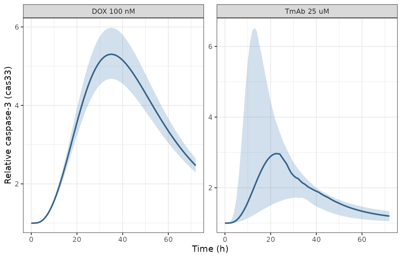
Median and 5th-95th percentile of relative caspase-3 across 100 virtual treatment groups per condition (between-group variability on Sc1 and Sc2; no residual error).
# The caspase-3 peak rises monotonically with each group's slope, so the
# median of the per-group peaks tracks the typical-value peak.
grp_peaks <- sim_vpc |>
  dplyr::group_by(cond, id) |>
  dplyr::summarise(peak = max(cas33), .groups = "drop") |>
  dplyr::group_by(cond) |>
  dplyr::summarise(med_peak = stats::median(peak), .groups = "drop")
typ_tmab <- casp_peaks$cas33_peak[casp_peaks$group == "TmAb 25 uM"]
stopifnot(
  abs(grp_peaks$med_peak[grp_peaks$cond == "DOX 100 nM"] / dox_pk$cas33_peak - 1) < 0.10,
  abs(grp_peaks$med_peak[grp_peaks$cond == "TmAb 25 uM"] / typ_tmab - 1) < 0.25
)
In vitro AC16 viability (Figure 3)
Without drug, relative viability grows exponentially at the
first-order growth rate kg. Over 96 h it reaches exp(0.035
x 96) = 28.8, which sits on the published control fit.
viab_grid <- expand.grid(dox = c(0, 1.1, 10.5, 25), tmab_um = c(0, 13.3, 23, 28.4))
# Exact applied TmAb concentrations from the deposited Monolix code (nM).
tm_nm <- c(`0` = 0, `13.3` = 13330, `23` = 23000, `28.4` = 28380)
sim_viab <- purrr::map_dfr(seq_len(nrow(viab_grid)), function(i) {
  tm <- tm_nm[[as.character(viab_grid$tmab_um[i])]]
  ev <- make_group(viab_grid$dox[i], tm, seq(0, 96, by = 1), "cas92")
  as.data.frame(rxode2::rxSolve(typ_ac16, ev)) |>
    dplyr::mutate(dox = viab_grid$dox[i], tmab_um = viab_grid$tmab_um[i])
})
#> ℹ omega/sigma items treated as zero: 'etalsc1', 'etalsc2', 'etalkd2'
#> ℹ omega/sigma items treated as zero: 'etalsc1', 'etalsc2', 'etalkd2'
#> ℹ omega/sigma items treated as zero: 'etalsc1', 'etalsc2', 'etalkd2'
#> ℹ omega/sigma items treated as zero: 'etalsc1', 'etalsc2', 'etalkd2'
#> ℹ omega/sigma items treated as zero: 'etalsc1', 'etalsc2', 'etalkd2'
#> ℹ omega/sigma items treated as zero: 'etalsc1', 'etalsc2', 'etalkd2'
#> ℹ omega/sigma items treated as zero: 'etalsc1', 'etalsc2', 'etalkd2'
#> ℹ omega/sigma items treated as zero: 'etalsc1', 'etalsc2', 'etalkd2'
#> ℹ omega/sigma items treated as zero: 'etalsc1', 'etalsc2', 'etalkd2'
#> ℹ omega/sigma items treated as zero: 'etalsc1', 'etalsc2', 'etalkd2'
#> ℹ omega/sigma items treated as zero: 'etalsc1', 'etalsc2', 'etalkd2'
#> ℹ omega/sigma items treated as zero: 'etalsc1', 'etalsc2', 'etalkd2'
#> ℹ omega/sigma items treated as zero: 'etalsc1', 'etalsc2', 'etalkd2'
#> ℹ omega/sigma items treated as zero: 'etalsc1', 'etalsc2', 'etalkd2'
#> ℹ omega/sigma items treated as zero: 'etalsc1', 'etalsc2', 'etalkd2'
#> ℹ omega/sigma items treated as zero: 'etalsc1', 'etalsc2', 'etalkd2'
ggplot(sim_viab, aes(time, viability)) +
  geom_line(linewidth = 0.8, colour = "purple4") +
  facet_grid(paste("TmAb", tmab_um, "uM") ~ paste("DOX", dox, "nM"), scales = "free_y") +
  labs(x = "Time (h)", y = "Relative cell viability") +
  theme_bw(base_size = 9)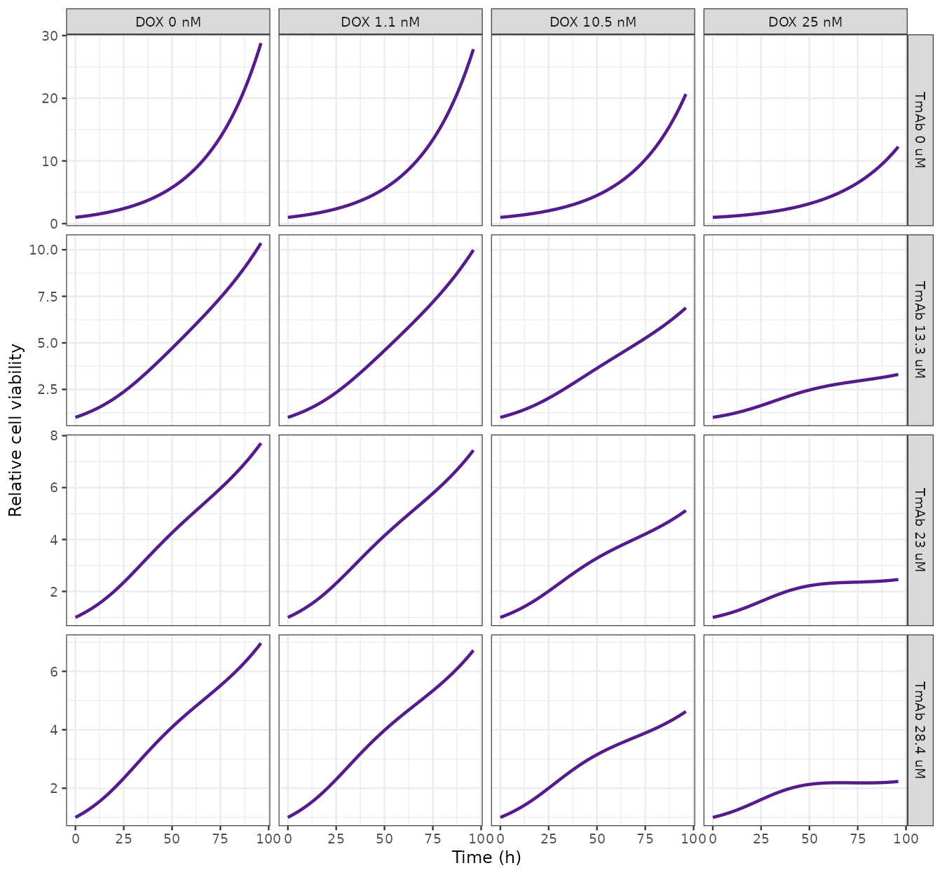
Replicates Figure 3 of Yu 2025: typical-value relative AC16 cell viability over 96 h for every DOX x TmAb condition of the viability experiment.
v96 <- sim_viab |>
  dplyr::filter(time == 96) |>
  dplyr::select(dox, tmab_um, viability)
v96 |>
  tidyr::pivot_wider(names_from = tmab_um, values_from = viability, names_prefix = "tmab_") |>
  dplyr::rename(
    "DOX (nM)" = dox, "TmAb 0 uM" = tmab_0, "TmAb 13.3 uM" = tmab_13.3,
    "TmAb 23 uM" = tmab_23, "TmAb 28.4 uM" = tmab_28.4
  ) |>
knitr::kable(digits = 2, caption = "Typical-value relative viability at 96 h.")| DOX (nM) | TmAb 0 uM | TmAb 13.3 uM | TmAb 23 uM | TmAb 28.4 uM |
|---|---|---|---|---|
| 0.0 | 28.79 | 10.35 | 7.71 | 6.96 |
| 1.1 | 27.83 | 9.99 | 7.44 | 6.72 |
| 10.5 | 20.66 | 6.88 | 5.12 | 4.63 |
| 25.0 | 12.27 | 3.30 | 2.46 | 2.23 |
ctl96 <- v96$viability[v96$dox == 0 & v96$tmab_um == 0]
stopifnot(
  # Control is pure exponential growth: R(96) = exp(kg * 96).
  abs(ctl96 / exp(0.035 * 96) - 1) < 1e-4,
  # Viability falls with DOX at every TmAb level and with TmAb at every DOX
  # level (the drug effects only ever slow growth or add death).
  all(tapply(v96$viability, v96$tmab_um, function(v) all(diff(v) < 0))),
  all(tapply(v96$viability, v96$dox, function(v) all(diff(v) < 0)))
)
The published Figure 3 curves are group-level fits, with
empirical-Bayes estimates on the DOX growth-inhibition slope
kd2 (omega 0.69) and on the caspase slopes. The
typical-value curves above therefore match the control panel and the
ordering of the panels, not each panel’s exact level. For example, the
typical DOX 25 nM group reaches 12.3 at 96 h, while the published fit
reaches about 18.
In vitro BNP release (Figure 4)
The BNP layer has no random effects, so its typical-value solution is the published fit itself.
bnp_groups <- data.frame(
  group = c("Control", "DOX 25 nM", "TmAb 23 uM", "DOX 25 nM + TmAb 23 uM"),
  dox = c(0, 25, 0, 25),
  tmab = c(0, 0, 23000, 23000)
)
sim_bnp <- purrr::map_dfr(seq_len(nrow(bnp_groups)), function(i) {
  ev <- make_group(bnp_groups$dox[i], bnp_groups$tmab[i], seq(0, 72, by = 0.25), "bnp3")
  as.data.frame(rxode2::rxSolve(typ_bnp, ev)) |>
    dplyr::mutate(group = bnp_groups$group[i])
})
sim_bnp$group <- factor(sim_bnp$group, levels = bnp_groups$group)
ggplot(sim_bnp, aes(time, bnp3)) +
  geom_line(linewidth = 0.9, colour = "purple4") +
  facet_wrap(~group, scales = "free_y") +
  labs(x = "Time (h)", y = "Relative BNP level") +
  theme_bw()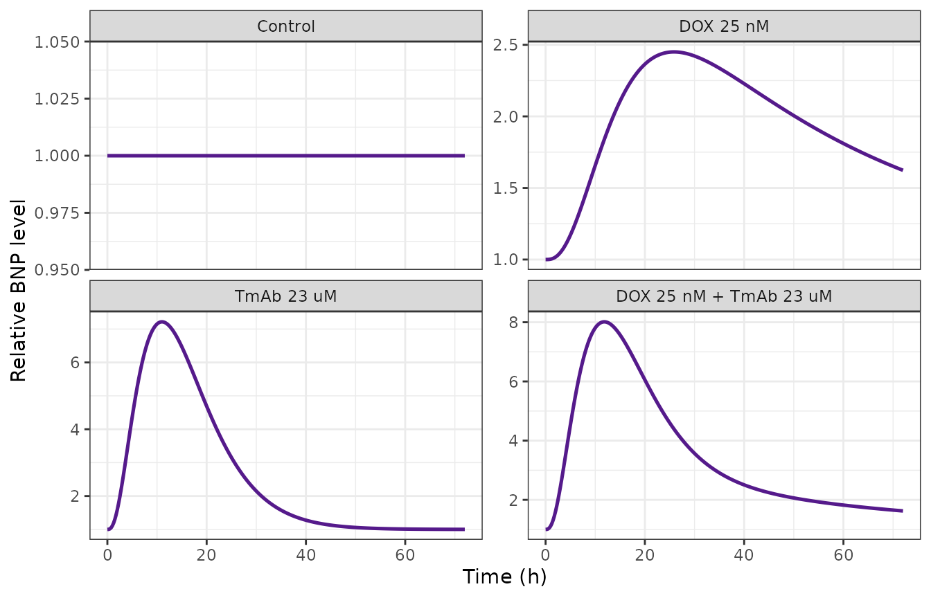
Replicates Figure 4 of Yu 2025: relative BNP in the AC16 culture supernatant over 72 h.
Peak values and timings read from the published Figure 4 fit curves:
bnp_pub <- data.frame(
  group = c("DOX 25 nM", "TmAb 23 uM", "DOX 25 nM + TmAb 23 uM"),
  pub_peak = c(2.45, 7.2, 7.9),
  pub_tpeak = c(27, 11, 12)
)
bnp_cmp <- sim_bnp |>
  dplyr::group_by(group) |>
  dplyr::summarise(sim_peak = max(bnp3), sim_tpeak = time[which.max(bnp3)], .groups = "drop") |>
  dplyr::mutate(group = as.character(group)) |>
  dplyr::inner_join(bnp_pub, by = "group") |>
  dplyr::mutate(pct_diff = 100 * (sim_peak / pub_peak - 1))
bnp_cmp |>
  dplyr::rename(
    "Group" = group, "Simulated peak" = sim_peak, "Simulated peak time (h)" = sim_tpeak,
    "Published peak" = pub_peak, "Published peak time (h)" = pub_tpeak, "Peak difference (%)" = pct_diff
  ) |>
knitr::kable(digits = 2, caption = "Typical-value BNP peaks against the digitised Figure 4 fits.")| Group | Simulated peak | Simulated peak time (h) | Published peak | Published peak time (h) | Peak difference (%) |
|---|---|---|---|---|---|
| DOX 25 nM | 2.45 | 25.75 | 2.45 | 27 | 0.01 |
| TmAb 23 uM | 7.22 | 11.00 | 7.20 | 11 | 0.23 |
| DOX 25 nM + TmAb 23 uM | 8.01 | 11.75 | 7.90 | 12 | 1.45 |
DOX degradation in the medium (PKNCA)
The only pharmacokinetic process in the in vitro models is first-order DOX loss from the culture medium. PKNCA recovers its half-life, log(2) / 0.022 = 31.5 h, for each applied concentration of the viability experiment:
dox_lvls <- c(1.1, 10.5, 25)
conc_df <- purrr::map_dfr(seq_along(dox_lvls), function(i) {
  ev <- make_group(dox_lvls[i], 0, seq(0, 96, by = 2), "cas92", id = i)
  as.data.frame(rxode2::rxSolve(typ_ac16, ev, returnType = "data.frame")) |>
    dplyr::mutate(id = i, treatment = paste("DOX", dox_lvls[i], "nM"))
}) |>
  dplyr::filter(!is.na(conc_dox)) |>
  dplyr::distinct(id, time, .keep_all = TRUE) |>
  dplyr::transmute(id, time, Cc = conc_dox, treatment)
#> ℹ omega/sigma items treated as zero: 'etalsc1', 'etalsc2', 'etalkd2'
#> ℹ omega/sigma items treated as zero: 'etalsc1', 'etalsc2', 'etalkd2'
#> ℹ omega/sigma items treated as zero: 'etalsc1', 'etalsc2', 'etalkd2'
dose_df <- data.frame(
  id = seq_along(dox_lvls), time = 0, amt = dox_lvls,
  treatment = paste("DOX", dox_lvls, "nM")
)
nca <- PKNCA::pk.nca(PKNCA::PKNCAdata(
  PKNCA::PKNCAconc(conc_df, Cc ~ time | treatment + id),
  PKNCA::PKNCAdose(dose_df, amt ~ time | treatment + id, route = "intravascular"),
  intervals = data.frame(start = 0, end = 96, cmax = TRUE, half.life = TRUE)
))
nca_tbl <- as.data.frame(nca$result) |>
  dplyr::filter(PPTESTCD %in% c("cmax", "half.life")) |>
  dplyr::select(treatment, PPTESTCD, PPORRES) |>
  tidyr::pivot_wider(names_from = PPTESTCD, values_from = PPORRES)
nca_tbl |>
  dplyr::rename("Treatment" = treatment, "Cmax (nM)" = cmax, "t1/2 (h)" = half.life) |>
knitr::kable(digits = 2, caption = "PKNCA DOX medium-concentration metrics.")| Treatment | Cmax (nM) | t1/2 (h) |
|---|---|---|
| DOX 1.1 nM | 1.1 | 31.51 |
| DOX 10.5 nM | 10.5 | 31.51 |
| DOX 25 nM | 25.0 | 31.51 |
Clinical BNP scale-up (Figures 5 and 6)
The clinical model is the in vitro BNP chain without the decaying
TmAb stimulus. The trastuzumab cardiac interstitial concentration enters
as a time-varying covariate, CP_TRASTUZUMAB_NM (nM), and
the TmAb slope is scaled by fSct = 0.86. The paper
generated that concentration with the Glassman and Balthasar 2016 human
mAb PBPK model. Neither the PBPK model nor the simulated cardiac profile
is published with Yu 2025, and no trastuzumab model in nlmixr2lib
produces a cardiac interstitial concentration. Figures 5 and 6 therefore
cannot be replicated here: users supply their own interstitial
trajectory.
With a constant driver C switched on at t = 0, the
three-compartment chain has a closed-form solution. With
A = fSct x Sbnp2 x C and k = kbnp, it is
BNP3(t) = 1 + A (1 - exp(-k t) (1 + k t + (k t)^2 / 2)), so
the relative BNP settles at 1 + A. The check below confirms
that the packaged model reproduces this solution.
hum_levels <- c(10, 40, 80)
t_h <- seq(0, 96, by = 0.5)
sim_hum <- purrr::map_dfr(seq_along(hum_levels), function(i) {
  ev <- data.frame(
    id = i, time = t_h, evid = 0L, amt = 0, cmt = "bnp3",
    CP_TRASTUZUMAB_NM = hum_levels[i], CP_DOXORUBICIN_NGML = 0
  )
  as.data.frame(rxode2::rxSolve(typ_hum, ev, atol = 1e-10, rtol = 1e-10)) |>
    dplyr::mutate(id = i, conc = hum_levels[i])
})
k <- 0.202
sim_hum <- sim_hum |>
  dplyr::mutate(
    A = 0.86 * 0.005 * conc,
    closed = 1 + A * (1 - exp(-k * time) * (1 + k * time + (k * time)^2 / 2))
  )
ggplot(sim_hum, aes(time, bnp3, colour = factor(conc))) +
  geom_line(linewidth = 0.9) +
  geom_line(aes(y = closed), linetype = "dashed", colour = "black") +
  labs(x = "Time (h)", y = "Relative BNP", colour = "Cardiac ISF TmAb (nM)") +
  theme_bw()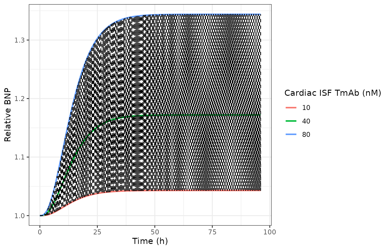
Relative BNP under constant cardiac interstitial trastuzumab concentrations (closed form as dashed lines).
The steady-state relation gives a sense of scale. The Figure 5 fit peaks at a relative BNP of about 1.33 after the 8 mg/kg loading dose. If the driver were a plateau, that peak would correspond to a cardiac interstitial concentration of 0.33 / (0.86 x 0.005), or about 77 nM. At about 148 kDa for trastuzumab, that is roughly 11 ug/mL.
Assumptions and deviations
-
Caspase-3 input (Eq 5). The printed Eq 5 multiplies
the caspase-3 production term by
Cas9S. The deposited Monolix code, in both supplement files, does not:ddt_Cas31 = Kcas3*Cas92^c3 - Kcas3*Cas31. The packaged model follows the code. With the printed form, the typical TmAb 25 uM caspase-3 response rises to about 11.5 and is still near 10.7 at 72 h. The published Figure 2 fit peaks near 4.2 and falls back towards 1. The maintainers checked both forms by simulation. -
Scaled table units. Table 1 reports
Sc1in units of 10^-2 nM^-1 andkcas9sin units of 10^-3 h^-1. The packaged values are 0.046 x 10^-2 and 0.093 x 10^-3. With these values the DOX 100 nM caspase peaks reproduce Figure 2 (1.45 against 1.45, and 5.3 against 5.4). The unscaled values would put the DOX caspase-9 stimulus about 100-fold higher. -
BNP turnover. Table 1 prints
k bnp = 0.20 (fix). The deposited code usesKbnp = 0.202, which is the value packaged. - Omega is an SD. Monolix reports omega as the SD of eta. The %CV column of Table 1 equals sqrt(exp(omega^2) - 1) for all three random effects (0.049 -> 5%, 0.99 -> 129%, 0.69 -> 78%), so the packaged variances are omega^2.
- Between-group, not between-subject, variability. Each Monolix “individual” was a treatment group. The two caspase slopes carry variability in the protein-dynamics fit, and the DOX growth-inhibition slope carries it in the viability fit. The packaged model carries all three on one coupled system. The paper fixed the protein-dynamics estimates (population values and omegas) before fitting the death layer.
-
Rise of caspase-3 floored at zero. Eq 8 raises
Cas33 - 1to the non-integer powerc4 = 1.5. The packaged model usesmax(cas33 - 1, 0)so the death signal stays real if caspase-3 dips below baseline. With the published parameters caspase-3 never falls below 1, so this changes no published simulation. - TmAb held constant in the caspase and viability layers. As in the deposited code, TmAb enters as a constant medium concentration, with no loss in these two layers. In the BNP layer, a separate hypothetical stimulus compartment starts at the applied concentration and decays first-order (Eq 12).
- In vitro TmAb concentrations. The applied TmAb concentrations are the exact values in the deposited code (13,330, 23,000 and 28,380 nM), which the paper’s text rounds to 13.3, 23 and 28.4 uM.
-
Doxorubicin in the human model. The deposited human
code carries
Cdox(nM) as a regressor. All of the paper’s clinical data are trastuzumab monotherapy, soCdoxwas 0 in every published fit. The packaged model takes the registeredCP_DOXORUBICIN_NGML(ng/mL) and converts it to nM with the doxorubicin molar mass of 543.52 g/mol. The source states neither the molar mass nor the matrix ofCdox. -
Single-output observation name. The two BNP models
observe
bnp3, the paper’s own name for the measured compartment (Figure 1). nlmixr2lib has no registered canonical for a relative-BNP output, so the convention check warns on that name.