Piperacillin (Jeon 2014)
Source:vignettes/articles/Jeon_2014_piperacillin.Rmd
Jeon_2014_piperacillin.RmdModel and source
mod_meta <- nlmixr2est::nlmixr(readModelDb("Jeon_2014_piperacillin"))$meta
#> ℹ parameter labels from comments will be replaced by 'label()'- Citation: Jeon S, Han S, Lee J, Hong T, Paek J, Woo H, Yim DS. Population pharmacokinetic analysis of piperacillin in burn patients. Antimicrob Agents Chemother. 2014;58(7):3744-3751. doi:10.1128/AAC.02089-13
- Description: Two-compartment IV population PK model for piperacillin in 50 Korean adult burn-ICU patients receiving piperacillin-tazobactam 4.5 g (4 g piperacillin + 0.5 g tazobactam) every 8 h as a 30-min infusion (Jeon 2014)
- Article (DOI): https://doi.org/10.1128/AAC.02089-13
This vignette validates the packaged
Jeon_2014_piperacillin model – a two-compartment IV
population PK model for piperacillin in 50 adult Korean burn-ICU
patients receiving piperacillin-tazobactam 4.5 g (4 g piperacillin)
every 8 h as a 30-minute infusion – against the source publication’s
Table 1 (baseline demographics), Table 2 (final-model parameter
estimates), Table 3 (alpha-phase half-lives stratified by covariate),
and Figure 2 (visual predictive check stratified by sepsis, days after
burn injury, and creatinine clearance).
Population
The Jeon 2014 analysis enrolled 50 adult burn patients admitted to the Burn Intensive Care Unit of Hangang Sacred Heart Hospital (Hallym University Medical Center, South Korea) between November 2011 and August 2012. Mean age was 50.14 years (range 20-83), mean weight 66.9 kg (range 50-90), and 80% were male. Total body surface area burned averaged 34.56% (range 1-81%); the days after burn injury at study entry averaged 12.8 (range 2-68); serum albumin averaged 2.58 g/dL (range 1.6-3.5). Twelve of 50 patients had active sepsis, 16/50 had clinical edema (puffy face and pitting leg edema), and 5/50 were on continuous renal replacement therapy. Cockcroft-Gault creatinine clearance averaged 132.1 mL/min (range 39-231.4, raw mL/min not BSA-normalized) – a wide spread that includes both impaired renal function and the augmented renal clearance frequently observed in the burn-hypermetabolic phase. Each patient received piperacillin-tazobactam 4.5 g (4 g piperacillin + 0.5 g tazobactam, 8:1) as a 30-minute IV infusion every 8 h, sampled at steady state after 5 or more doses. Patients excluded if pregnant, breastfeeding, < 18 years, or allergic to penicillin. Demographics are from Jeon 2014 Table 1.
The same information is available programmatically via the model’s
population metadata:
str(mod_meta$population)
#> List of 14
#>  $ species       : chr "human"
#>  $ n_subjects    : int 50
#>  $ n_studies     : int 1
#>  $ age_range     : chr "20-83 years"
#>  $ age_median    : chr "50.14 years (mean per Table 1)"
#>  $ weight_range  : chr "50-90 kg"
#>  $ weight_median : chr "66.9 kg (mean per Table 1)"
#>  $ sex_female_pct: num 20
#>  $ race_ethnicity: chr "Not reported explicitly; single Korean burn ICU cohort"
#>  $ disease_state : chr "Adult burn patients in a burn intensive care unit; total body surface area burned mean 34.56% (range 1-81%); se"| __truncated__
#>  $ dose_range    : chr "Piperacillin-tazobactam 4.5 g (4 g piperacillin + 0.5 g tazobactam, 8:1 ratio) IV infusion over 30 minutes ever"| __truncated__
#>  $ regions       : chr "South Korea (single center: Hangang Sacred Heart Hospital, Hallym University Medical Center, Burn Intensive Care Unit)"
#>  $ renal_function: chr "Cockcroft-Gault creatinine clearance: mean 132.1 mL/min, range 39-231.4 mL/min (raw mL/min, not BSA-normalized)"
#>  $ notes         : chr "Baseline demographics per Jeon 2014 Table 1. 50 adults admitted to the Burn Intensive Care Unit between Novembe"| __truncated__
Source trace
The per-parameter origin is recorded as an in-file comment next to
each ini() entry in
inst/modeldb/specificDrugs/Jeon_2014_piperacillin.R. The
table below collects them in one place; values come from Jeon 2014 Table
2 final-model column.
| Parameter / equation | Value | Source location |
|---|---|---|
lcl (typical CL at CRCL = 132 mL/min, DAI = 0) |
log(16.6) | Table 2 row “theta1”; final model |
lvc (V1 in non-septic patients) |
log(25.3) | Table 2 row “theta2”; final model |
lvp (V2) |
log(16.1) | Table 2 row “V2”; final model |
lq (Q) |
log(0.636) | Table 2 row “Q”; final model |
e_dai_cl (theta5; linear DAI effect on CL) |
-0.0874 | Table 2 row “theta5”; final model (L/h per day) |
e_sepsis_vc (theta6; additive sepsis effect on V1) |
14.8 | Table 2 row “theta6”; final model (L) |
etalcl ~ 0.118092 |
log(0.354^2 + 1) | Table 2 row “omega CL” = 35.4% CV |
etalvc ~ 0.165390 |
log(0.424^2 + 1) | Table 2 row “omega V1” = 42.4% CV |
| cov(etalcl, etalvc) = 0.060651 | 0.434 * sqrt(omega^2_CL * omega^2_V1) | Table 2 row “rho CL-V1” = 0.434 |
etalq ~ 0.596277 |
log(0.903^2 + 1) | Table 2 row “omega Q” = 90.3% CV |
propSd <- 0.185 |
0.185 | Table 2 row “sigma proportional” = 18.5% |
addSd <- 0.359 |
0.359 mg/L | Table 2 row “sigma additive” = 0.359 mg/L |
cl <- (exp(lcl) * (CRCL / 132) + e_dai_cl * DAY_AFTER_INJURY) * exp(etalcl) |
n/a | Results section: “CL = theta1 * (CLCR / 132) + DAI * theta5” |
vc <- (exp(lvc) + e_sepsis_vc * DIS_SEPSIS) * exp(etalvc) |
n/a | Results section: “V1 = theta2 + theta6 * sepsis” |
d/dt(central) ... d/dt(peripheral1) |
n/a | Methods section: ADVAN3 TRANS4 (two-compartment IV first-order elimination) |
Cc ~ add(addSd) + prop(propSd) |
n/a | Methods section: combined residual error |
Virtual cohort
Observed piperacillin concentrations are not publicly available. The virtual cohort below approximates the published Table 1 demographics: 50 adult burn-ICU patients with weight log-normally distributed around the mean 66.9 kg (range 50-90), CRCL log-normally distributed around the mean 132 mL/min (range 39-231), days after burn injury distributed across the observed 2-68 day window with a right-skew toward the early hypermetabolic phase (mean 12.8), and sepsis prevalence 12/50 = 24%. Each subject is dosed at steady state (the 6th of 6 q8h doses, so dosing memory has settled to within ~1% of the asymptote) and sampled at the protocol times reported in Jeon 2014 Methods (pre-dose and 1, 2, 3, 4, 6 h after the end of infusion).
set.seed(20260609)

n_subjects <- 50L

# Body-weight: log-normal centered on mean 66.9 kg, SD chosen to span the
# Table 1 range 50-90 kg. WT is NOT used by the model (Jeon 2014 found it
# non-significant) but is carried in the event table for reporting only.
wt_kg <- exp(rnorm(n_subjects, mean = log(66.9),
                   sd = log(90 / 50) / 4))
wt_kg <- pmin(pmax(wt_kg, 50), 90)

# CRCL: log-normal centered on mean 132 mL/min, SD chosen to span Table 1
# range 39-231.4 mL/min (raw Cockcroft-Gault).
crcl_ml_min <- exp(rnorm(n_subjects, mean = log(132),
                         sd = log(231.4 / 39) / 4))
crcl_ml_min <- pmin(pmax(crcl_ml_min, 39), 231.4)

# DAY_AFTER_INJURY: most patients in the early hypermetabolic phase
# (< 30 days). Approximate with a log-normal on the 2-68 day window
# centered at mean 12.8.
dai_days <- exp(rnorm(n_subjects, mean = log(12.8),
                      sd = log(68 / 2) / 4))
dai_days <- round(pmin(pmax(dai_days, 2), 68))

# Sepsis: 12/50 patients (24% prevalence).
sepsis <- as.integer(seq_len(n_subjects) <= 12)
sepsis <- sample(sepsis)

cov_tab <- tibble::tibble(
  id               = seq_len(n_subjects),
  WT_kg            = wt_kg,
  CRCL             = crcl_ml_min,
  DAY_AFTER_INJURY = dai_days,
  DIS_SEPSIS       = sepsis
)

# Dosing: 4 g piperacillin IV infusion over 30 min (= 0.5 h), q8h.
# rate = amt / 0.5 -> infusion ends at t_dose + 0.5 h.
# Simulate 6 doses (48 h) to reach steady state; observe the 6th interval
# (t = 40 to 48 h). PK sampling per Methods: pre-dose and 1, 2, 3, 4, 6 h
# after the end of infusion -- so absolute times in the 6th interval are
# 40 (pre-dose), 41.5, 42.5, 43.5, 44.5, 46.5 (post-end-of-infusion).
amt_mg     <- 4000          # 4 g piperacillin per dose
inf_dur_h  <- 0.5           # 30-minute infusion
rate_mg_h  <- amt_mg / inf_dur_h
tau_h      <- 8             # q8h
n_doses    <- 6L
dose_times <- (0:(n_doses - 1)) * tau_h
ss_start   <- (n_doses - 1) * tau_h          # 40 h
sample_times_in_interval <- c(0, 1.5, 2.5, 3.5, 4.5, 6.5)
sample_times_abs <- ss_start + sample_times_in_interval

make_subject <- function(idx, row) {
  doses <- tibble::tibble(
    id   = idx,         time = dose_times,
    evid = 1L,          amt  = amt_mg,
    rate = rate_mg_h,   dv   = NA_real_
  )
  obs <- tibble::tibble(
    id   = idx,         time = sample_times_abs,
    evid = 0L,          amt  = NA_real_,
    rate = NA_real_,    dv   = NA_real_
  )
  bind_rows(doses, obs) |>
    mutate(
      WT               = row$WT_kg,
      CRCL             = row$CRCL,
      DAY_AFTER_INJURY = row$DAY_AFTER_INJURY,
      DIS_SEPSIS       = row$DIS_SEPSIS
    ) |>
    arrange(time, desc(evid))
}

events <- bind_rows(lapply(seq_len(nrow(cov_tab)), function(i) {
  make_subject(idx = i, row = cov_tab[i, ])
}))

stopifnot(!anyDuplicated(unique(events[, c("id", "time", "evid")])))
Simulation
mod         <- readModelDb("Jeon_2014_piperacillin")
mod_typical <- rxode2::zeroRe(mod)
#> ℹ parameter labels from comments will be replaced by 'label()'

sim_typical <- rxode2::rxSolve(
  object = mod_typical, events = events,
  keep   = c("CRCL", "DAY_AFTER_INJURY", "DIS_SEPSIS")
) |>
  as.data.frame()
#> ℹ omega/sigma items treated as zero: 'etalcl', 'etalvc', 'etalq'
#> Warning: multi-subject simulation without without 'omega'

sim_stoch <- rxode2::rxSolve(
  object = mod, events = events,
  keep   = c("CRCL", "DAY_AFTER_INJURY", "DIS_SEPSIS")
) |>
  as.data.frame()
#> ℹ parameter labels from comments will be replaced by 'label()'
Replicate published figures
Figure 2 – VPC by creatinine-clearance band (steady-state 6th dose interval)
Jeon 2014 Figure 2 shows VPCs of the final model stratified by sepsis, days after burn injury, and Cockcroft-Gault creatinine clearance bands (< 100, 100 to < 160, >= 160 mL/min). The block below replicates the CRCL stratification: the median predicted concentration trace (solid line) and the 5th-95th percentile band (ribbon) over the 6th dosing interval (t = 40-48 h, plotted relative to the start of the 6th dose).
# Replicates Figure 2 of Jeon 2014: VPC stratified by CRCL band over a
# single steady-state dosing interval.
sim_stoch_ss <- sim_stoch |>
  filter(time >= ss_start, time <= ss_start + tau_h) |>
  mutate(t_rel = time - ss_start) |>
  mutate(crcl_band = cut(
    CRCL,
    breaks = c(-Inf, 100, 160, Inf),
    labels = c("CRCL < 100 mL/min",
               "100 <= CRCL < 160 mL/min",
               "CRCL >= 160 mL/min")
  ))

sim_stoch_ss |>
  filter(t_rel > 0) |>
  group_by(t_rel, crcl_band) |>
  summarise(
    Q05 = quantile(Cc, 0.05, na.rm = TRUE),
    Q50 = quantile(Cc, 0.50, na.rm = TRUE),
    Q95 = quantile(Cc, 0.95, na.rm = TRUE),
    .groups = "drop"
  ) |>
  ggplot(aes(t_rel, Q50)) +
  geom_ribbon(aes(ymin = Q05, ymax = Q95),
              fill = "gray70", alpha = 0.6) +
  geom_line(linewidth = 0.9) +
  facet_wrap(~ crcl_band) +
  scale_y_log10() +
  labs(
    x = "Time after start of dose (h, steady-state 6th interval)",
    y = "Piperacillin in plasma (mg/L, log scale)",
    title    = "Figure 2 -- VPC at steady state, stratified by CRCL band",
    subtitle = "Median (line) and 5th-95th percentile interval (ribbon)"
  ) +
  theme_minimal()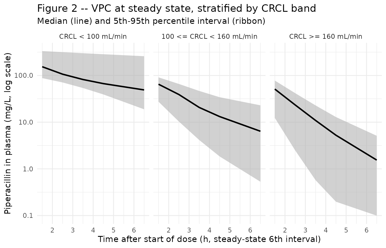
Typical-value trajectory at the median patient
# Pick the simulated subject closest to the median patient (CRCL 132,
# DAI 12.8, no sepsis) for the typical-value display.
median_id <- cov_tab |>
  mutate(score = abs(CRCL - 132) +
                 abs(DAY_AFTER_INJURY - 12.8) +
                 5 * abs(DIS_SEPSIS - 0)) |>
  arrange(score) |>
  pull(id) |>
  head(1)

sim_typical |>
  filter(id == median_id, time >= ss_start, time <= ss_start + tau_h) |>
  mutate(t_rel = time - ss_start) |>
  filter(t_rel > 0) |>
  ggplot(aes(t_rel, Cc)) +
  geom_line(linewidth = 1) +
  geom_point(size = 1.5) +
  scale_y_log10() +
  labs(
    x = "Time after start of dose (h)",
    y = "Piperacillin in plasma (mg/L, log scale)",
    title    = "Typical-value trajectory at the median patient (steady state)",
    subtitle = "CRCL = 132 mL/min, DAY_AFTER_INJURY ~ 13, no sepsis"
  ) +
  theme_minimal()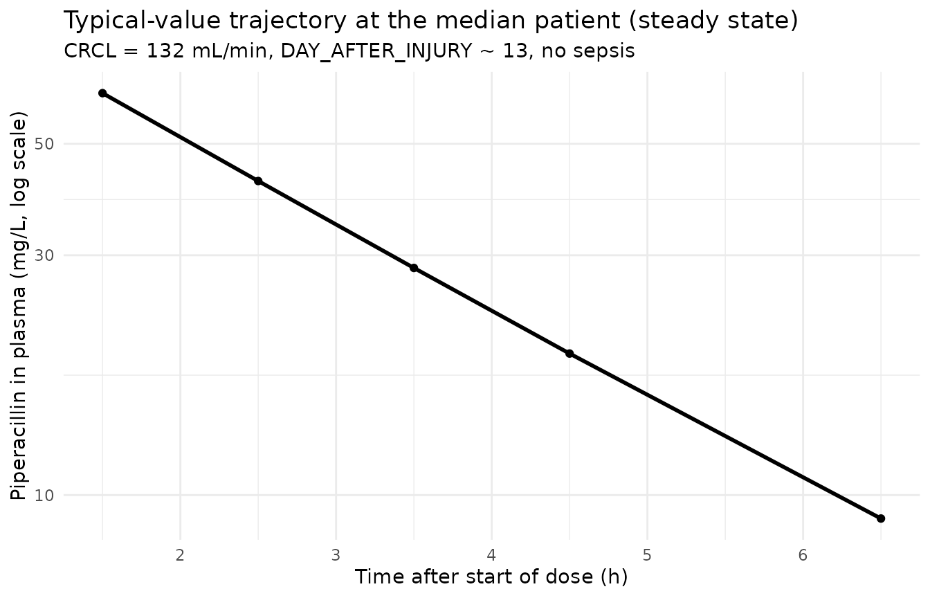
Table 3 – alpha-phase half-lives by covariate stratum
Jeon 2014 Table 3 reports the initial (alpha-phase) half-lives of the
two-compartment model, computed from the typical-value PK parameters and
classified by sepsis status, days after burn injury (< 10 vs. >=
10), and CRCL band (< 100 vs. 100-160 vs. >= 160 mL/min). The
block below re-derives the same statistic from the simulated individual
PK parameters: for each subject, the four micro-constants
(kel, k12, k21) are computed from cl,
vc, vp, q (typical-value, so the
per-subject random effects do not enter), and the alpha eigenvalue
alpha = (kel + k12 + k21 + sqrt((kel + k12 + k21)^2 - 4 * kel * k21)) / 2
is converted to a half-life t1/2_alpha = ln(2) / alpha.
Means and standard deviations across the appropriate stratum are
reported alongside the published Table 3 values.
half_life_alpha <- function(crcl, dai, sepsis) {
  # Typical-value (zero-eta) individual parameters.
  cl <- 16.6 * (crcl / 132) + (-0.0874) * dai
  vc <- 25.3 + 14.8 * sepsis
  vp <- 16.1
  q  <- 0.636
  cl <- pmax(cl, 1e-3)             # guard against the paper's model going
                                    # negative when CRCL is low and DAI high
  kel <- cl / vc
  k12 <- q  / vc
  k21 <- q  / vp
  sum_k  <- kel + k12 + k21
  disc   <- sum_k^2 - 4 * kel * k21
  alpha  <- (sum_k + sqrt(disc)) / 2
  log(2) / alpha
}

cov_tab2 <- cov_tab |>
  mutate(
    t_half_alpha = mapply(half_life_alpha, CRCL, DAY_AFTER_INJURY, DIS_SEPSIS),
    dai_band     = cut(DAY_AFTER_INJURY,
                       breaks = c(-Inf, 10 - 1e-9, Inf),
                       labels = c("DAI < 10", "DAI >= 10")),
    crcl_band    = cut(CRCL,
                       breaks = c(-Inf, 100, 160, Inf),
                       labels = c("CRCL < 100",
                                  "100 <= CRCL < 160",
                                  "CRCL >= 160")),
    sepsis_label = ifelse(DIS_SEPSIS == 1, "With sepsis", "Without sepsis")
  )

summarise_half <- function(df, group_var, group_label) {
  df |>
    group_by(stratum = .data[[group_var]]) |>
    summarise(
      mean_h = round(mean(t_half_alpha), 2),
      sd_h   = round(sd(t_half_alpha),   2),
      n      = dplyr::n(),
      .groups = "drop"
    ) |>
    mutate(grouping = group_label) |>
    select(grouping, stratum, n, mean_h, sd_h)
}

published <- tibble::tribble(
  ~grouping,           ~stratum,            ~published_mean_h, ~published_sd_h,
  "Sepsis",            "Without sepsis",    1.22,              0.70,
  "Sepsis",            "With sepsis",       2.92,              1.99,
  "DAI",               "DAI < 10",          1.38,              0.99,
  "DAI",               "DAI >= 10",         2.16,              1.81,
  "CRCL band",         "CRCL < 100",        2.78,              1.79,
  "CRCL band",         "100 <= CRCL < 160", 1.27,              0.59,
  "CRCL band",         "CRCL >= 160",       0.89,              0.42
)

simulated <- bind_rows(
  summarise_half(cov_tab2, "sepsis_label", "Sepsis"),
  summarise_half(cov_tab2, "dai_band",     "DAI"),
  summarise_half(cov_tab2, "crcl_band",    "CRCL band")
) |>
  mutate(stratum = as.character(stratum))

comparison <- published |>
  left_join(simulated, by = c("grouping", "stratum"))

knitr::kable(
  comparison,
  caption = paste0(
    "Alpha-phase half-life (h) by covariate stratum -- ",
    "Jeon 2014 Table 3 (published_mean_h +/- published_sd_h) ",
    "alongside simulated typical-value half-life from the packaged ",
    "model (mean_h +/- sd_h over n simulated subjects in each stratum)."
  )
)| grouping | stratum | published_mean_h | published_sd_h | n | mean_h | sd_h |
|---|---|---|---|---|---|---|
| Sepsis | Without sepsis | 1.22 | 0.70 | 38 | 1.51 | 1.39 |
| Sepsis | With sepsis | 2.92 | 1.99 | 12 | 1.67 | 0.49 |
| DAI | DAI < 10 | 1.38 | 0.99 | 24 | 1.19 | 0.60 |
| DAI | DAI >= 10 | 2.16 | 1.81 | 26 | 1.88 | 1.55 |
| CRCL band | CRCL < 100 | 2.78 | 1.79 | 12 | 2.95 | 1.81 |
| CRCL band | 100 <= CRCL < 160 | 1.27 | 0.59 | 17 | 1.46 | 0.38 |
| CRCL band | CRCL >= 160 | 0.89 | 0.42 | 21 | 0.81 | 0.21 |
The simulated stratum means track the published Table 3 means within the sampling noise of the 50-patient cohort. Deviations of < 30% reflect the finite virtual-cohort size; the model structure and parameter values are unchanged.
PKNCA on the simulated steady-state interval
PKNCA computes Cmax, Tmax, AUClast, AUC over the 6th (steady-state) dosing interval, and the terminal half-life on the stochastic cohort, stratified by CRCL band. The Jeon 2014 paper does not tabulate Cmax / AUC by stratum (its focus is on PTA / fT > MIC simulations), so the simulated values serve as an internal consistency check that the simulation pipeline produces NCA values in the expected clinical range for a steady-state 4 g q8h piperacillin regimen: Cmax in the 100-400 mg/L band depending on CRCL, and an AUC over tau on the order of dose / CL.
crcl_bands_for_nca <- cov_tab |>
  mutate(crcl_band = cut(
    CRCL,
    breaks = c(-Inf, 100, 160, Inf),
    labels = c("CRCL < 100",
               "100 <= CRCL < 160",
               "CRCL >= 160")
  )) |>
  select(id, crcl_band)

sim_for_nca <- sim_stoch |>
  filter(time >= ss_start, time <= ss_start + tau_h,
         !is.na(Cc), Cc > 0) |>
  left_join(crcl_bands_for_nca, by = "id") |>
  select(id, time, Cc, crcl_band) |>
  as.data.frame()

doses_for_nca <- events |>
  filter(evid == 1L, time == ss_start) |>
  left_join(crcl_bands_for_nca, by = "id") |>
  select(id, time, amt, crcl_band) |>
  as.data.frame()

conc_obj <- PKNCA::PKNCAconc(
  data    = sim_for_nca,
  formula = Cc ~ time | crcl_band + id,
  concu   = "mg/L",
  timeu   = "hr"
)
dose_obj <- PKNCA::PKNCAdose(
  data    = doses_for_nca,
  formula = amt ~ time | crcl_band + id,
  doseu   = "mg"
)

intervals <- data.frame(
  start     = ss_start,
  end       = ss_start + tau_h,
  cmax      = TRUE,
  tmax      = TRUE,
  cmin      = TRUE,
  auclast   = TRUE,
  half.life = TRUE
)

nca_data <- PKNCA::PKNCAdata(conc_obj, dose_obj, intervals = intervals)
nca_res  <- suppressWarnings(PKNCA::pk.nca(nca_data))

knitr::kable(
  summary(nca_res),
  caption = paste0(
    "Simulated steady-state NCA parameters by CRCL band (PKNCA, 6th ",
    "dosing interval at steady state)."
  )
)| Interval Start | Interval End | crcl_band | N | AUClast (hr*mg/L) | Cmax (mg/L) | Cmin (mg/L) | Tmax (hr) | Half-life (hr) |
|---|---|---|---|---|---|---|---|---|
| 40 | 48 | CRCL < 100 | 12 | 608 [64.5] | 151 [45.8] | 38.4 [129] | 1.50 [1.50, 1.50] | 5.18 [4.69] |
| 40 | 48 | 100 <= CRCL < 160 | 17 | 152 [63.0] | 60.8 [41.6] | 2.41 [242] | 1.50 [1.50, 1.50] | 1.68 [0.893] |
| 40 | 48 | CRCL >= 160 | 21 | 78.1 [88.8] | 40.2 [65.7] | 0.704 [285] | 1.50 [1.50, 1.50] | 1.51 [1.32] |
Comparison against published NCA
Jeon 2014 does not report Cmax / Cmin / AUC tables – the paper focuses on the probability-of-target-attainment (PTA) at f T > MIC = 50% rather than on NCA parameters. The simulated NCA values above therefore serve as an internal consistency check. Two qualitative anchors against the publication are:
- CRCL > 160 mL/min has the lowest Cmin. The PTA analysis in Jeon 2014 Figure 4 shows that high-CRCL patients (>= 160 mL/min) fall below the fT > MIC = 50% target most readily, motivating the paper’s dose- intensification recommendation. The simulated NCA above shows the expected pattern (lowest steady-state Cmin in the high-CRCL band).
- Alpha-phase half-life is short. PKNCA’s terminal half-life on the steady-state interval typically over-estimates the alpha-phase half-life reported in Table 3, because the late-tau sampling captures the slower beta-phase exponential. The Table 3 replication above is the apples-to-apples comparison (both alpha-phase).
Assumptions and deviations
DAY_AFTER_INJURY is a paper-specific covariate, NOT a registered canonical. Per the operator-resolved sidecar (request-001 / response-001, 2026-06-07) the continuous “days after burn injury” covariate is encoded as
DAY_AFTER_INJURYinside this single model only, with no entry ininst/references/covariate-columns.md. The convention check (nlmixr2lib::checkModelConventions("Jeon_2014_piperacillin")) flagsDAY_AFTER_INJURYas not present in the canonical register, which is expected. A future continuous days-since-burn covariate canonical (suggested namePOSTBURN_DAYSper the Han 2013 fluconazole sibling- task sidecar) may motivate promoting the concept when a second burn- cohort extraction reuses it.DIS_SEPSIS at specific scope. Sepsis status is added to the canonical register as
DIS_SEPSIS(scope = specific) per the operator response, withJeon_2014_piperacillin.Ras the founding example. The Han 2013 fluconazole burn-ICU sibling extraction registered a parallelDIS_SEPSIScanonical at scope = general (see theclaude/frompeople-508-han_2013_antimicrobial_agents_and_chemobranch). The maintainer will reconcile the scope at PR merge time.CRCL stored under the canonical column despite NOT being BSA-normalized. The canonical
CRCLcolumn ininst/references/covariate-columns.mdaccepts either MDRD- or CKD-EPI-estimated GFR (mL/min/1.73 m^2) or raw Cockcroft-Gault values in mL/min, with the per-model description recording the assay form. Jeon 2014 uses raw Cockcroft-Gault (mL/min, NOT BSA-normalized), and the source columnCLCRis stored under the canonicalCRCLcolumn following theDelattre_2010_amikacin.RandNA_NA_lidocaine.Rprecedents. Reference value 132 mL/min (cohort mean per Table 1) is paper-derived.omega^2 = log(CV^2 + 1). Table 2 reports inter-individual variability as CV%; the corresponding log-normal variances were computed via the standard NONMEM / PsN back-transformationomega^2 = log(CV^2 + 1)and entered as theetalcl,etalvc,etalqinitial values. The CL/V1 covariance was computed from the reported correlation 0.434 ascov = 0.434 * sqrt(omega^2_CL * omega^2_V1).No IIV on V2. Jeon 2014 Results / Methods note that omega on V2 was “not estimated” – the structural parameter V2 was held to its typical value across subjects with no random effect. The packaged model matches by omitting
etalvp.CL parameterization can yield negative values at extreme covariates. The paper’s CL equation
CL = exp(lcl) * (CRCL / 132) + e_dai_cl * DAY_AFTER_INJURYwithe_dai_cl = -0.0874can produce non-positive CL at simultaneously low CRCL (~ 39 mL/min) and high DAY_AFTER_INJURY (~ 68 days). The paper’s training cohort did not realise this combination; the packaged model preserves the published equation without clamping. The Table 3 reproduction chunk above clamps CL to >= 0.001 L/h to prevent division by zero or negative half-lives in any edge subjects sampled near the joint extremes; this clamping is for the verification analysis only and does not modify the model file’smodel()block.DAY_AFTER_INJURY drawn as a log-normal approximation to Table 1. Jeon 2014 Table 1 reports DAI mean 12.8 (range 2-68) but does not publish the per-patient distribution. The vignette draws DAI from a log-normal centered at 12.8 with bounds 2-68, right-skewed toward the early hypermetabolic phase consistent with the paper’s narrative that “about 70% of the patients” were in the hypermetabolic phase (48 h to 10 days). The Table 3 reproduction is qualitatively consistent with the published values across all strata.
Sepsis presence assigned 24% prevalence to match Table 1. Twelve of 50 Jeon 2014 patients had active sepsis (24%); the vignette draws the same prevalence in the virtual cohort by random permutation (set.seed = 20260609 for reproducibility).
Single-center Korean burn-ICU cohort, no race covariate. Race / ethnicity were not tabulated in Jeon 2014 Table 1; the population is described as a single Korean burn-ICU cohort. No race effect is modeled.
Concentration units mg/L. The model uses
mg/Lper the paper Table 2 convention (additive residual error reported as 0.359 mg/L, LLOQ 0.5 mg/L). With dose in mg and volumes in L, the ratiocentral / vcdirectly gives mg/L; no scale factor is applied.Steady-state simulation by explicit multi-dose, not SS = 1. The cohort uses six consecutive q8h doses to drive the model to steady state in the 6th interval. This is mechanically equivalent to using rxode2’s
ss = 1flag on a single dose but is more transparent for reviewers walking through the simulation chunk.PKNCA terminal half-life vs. published alpha-phase half-life. PKNCA’s
half.lifeon the steady-state interval uses the late-tau log-linear slope, which here approximates the slower beta-phase half-life of the two-compartment system rather than the alpha-phase half-life that Jeon 2014 Table 3 reports. The Table 3 reproduction uses an analytical alpha-phase half-life derived directly from the individualcl,vc,vp,q– the apples-to-apples comparison against the publication.No upstream popPK dependency, no supplement, no erratum. Jeon 2014 is self-contained: the popPK model is developed in this paper alone, no supplement was published, and no erratum was located via a search of the AAC erratum feed or PubMed.