Model and source
ui <- rxode2::rxode(readModelDb("Zhou_2026_tacrolimus"))
#> ℹ parameter labels from comments will be replaced by 'label()'- Citation: Zhou Y, Zhou Z, Chen S, Zhu L, Yun Y, Yuan Y, Chen C, Zou J, Zhao J. An Integrated Population Pharmacokinetic and Machine Learning Model for Predicting Tacrolimus Exposure in Adult Patients with Nephrotic Syndrome. Drug Des Devel Ther. 2026;20:576598. doi:10.2147/DDDT.S576598. Parameter values are the ‘Final model’ Estimate column of Supplementary Table S1; the structural covariate equation is the displayed equation in Results, ‘Population Pharmacokinetic Model’.
- Description: One-compartment population PK model with first-order absorption and elimination for oral immediate-release tacrolimus in adult Chinese patients with nephrotic syndrome, built from steady-state trough (Cmin) therapeutic drug monitoring data. Because only troughs were available the absorption rate constant is fixed at a literature value. Apparent clearance CL/F carries two multiplicative covariate effects: a reduction with concomitant Wuzhi capsule and a reduction in CYP3A53/3 non-expressers; no covariate was retained on apparent volume of distribution. Exponential inter-individual variability on CL/F only, with a proportional residual error. This is the population PK half of a paper whose second half feeds the individual CL/F estimate into a machine-learning ensemble; only the pharmacokinetic model is represented here.
- Article: https://doi.org/10.2147/DDDT.S576598
- Supplement (Table S1, the parameter table): https://www.dovepress.com/article/supplementary_file/576598/576598_Supplementary%20Material%20%25288%2529.docx
Zhou 2026 is a two-part paper. The first part builds a conventional
one-compartment population PK model of oral tacrolimus from steady-state
trough therapeutic-drug-monitoring (TDM) data; the second part feeds
each subject’s individual CL/F estimate, as one feature
among nine, into a weighted voting ensemble of gradient-boosting
regressors (CatBoost / AdaBoost / GraBoost, 5:3:2) that predicts the
measured trough. Only the population PK half is represented in
this package. The machine-learning ensemble is a feature-based
regression with no differential-equation structure, so there is nothing
for rxode2 to integrate; its performance metrics are
reported in the paper’s Table 2 and Tables S2-S5 and are not
reproducible from published coefficients (the fitted ensemble is
distributed only as a Streamlit web application). This vignette
validates the PK model.
Population
The model was estimated from 141 adult patients with nephrotic syndrome contributing 410 steady-state trough samples, drawn at the First Affiliated Hospital of Xinjiang Medical University between January 2018 and December 2019 (the paper’s “internal dataset”; 182 consecutive patients were screened). A temporal external-validation set enrolled January 2020 to December 2023 contributed a further 12 patients and 41 samples.
Baseline characteristics come from Zhou 2026 Table 1, whose percentages are expressed per sample (N = 410) rather than per patient. Median age 44 years (IQR 31-53), median weight 71 kg (IQR 61-79), median BMI 24.4 kg/m^2, 58.5% male. The cohort is deliberately multi-ethnic: Han 67.1%, Kazakh or Uyghur 27.1%, Hui 4.6%, other 1.2%. CYP3A5 rs776746 genotype was 1/1 in 4.4%, 1/3 in 35.6% and 3/3 in 60.0% of samples, a distribution that satisfies Hardy-Weinberg equilibrium (Table 3: chi-squared 0.395, p = 0.821). Concomitant Wuzhi capsule was taken in 6.6% of samples.
Dosing was oral immediate-release tacrolimus capsules on an empty stomach, started at 0.05-0.1 mg/kg/day split into a morning and an evening dose and then titrated to TDM; the observed total daily dose was a median of 3.00 mg (IQR 3.00-4.00). Samples were taken after at least three days of continuous dosing. Median time on tacrolimus at sampling was 59 days (IQR 19-139).
TDM control in this cohort was loose, which matters for the validation below: against the 5-10 ng/mL target for adult nephrotic syndrome, 46.6% of samples were below the window, 49.3% within it and only 4.1% above it.
The same information is available programmatically:
str(ui$population)
#> List of 13
#>  $ species       : chr "human"
#>  $ n_subjects    : int 141
#>  $ n_studies     : int 1
#>  $ age_range     : chr "18 years and older; median 44 years (IQR 31-53)"
#>  $ age_median    : chr "44 years"
#>  $ weight_range  : chr "median 71 kg (IQR 61-79)"
#>  $ weight_median : chr "71 kg"
#>  $ sex_female_pct: num 41.5
#>  $ race_ethnicity: Named num [1:4] 67.1 27.1 4.6 1.2
#>   ..- attr(*, "names")= chr [1:4] "Han" "Kazakh/Uyghur" "Hui" "Other"
#>  $ disease_state : chr "Adult patients with nephrotic syndrome receiving oral immediate-release tacrolimus as immunosuppressive therapy"| __truncated__
#>  $ dose_range    : chr "Oral immediate-release tacrolimus capsules, initial total daily dose 0.05-0.1 mg/kg divided into a morning and "| __truncated__
#>  $ regions       : chr "Single centre, First Affiliated Hospital of Xinjiang Medical University, Urumqi, Xinjiang, People's Republic of China"
#>  $ notes         : chr "Retrospective cohort of 182 consecutive patients screened; 141 patients contributing 410 steady-state trough sa"| __truncated__
Source trace
The per-parameter origin is recorded as an in-file comment next to
each ini() entry in
inst/modeldb/specificDrugs/Zhou_2026_tacrolimus.R. The
table below collects them in one place. Every structural value comes
from the “Final model” Estimate column of Supplementary Table
S1; the covariate coding comes from the displayed equation in
Results, “Population Pharmacokinetic Model”.
| Equation / parameter | Value | Source location |
|---|---|---|
lka (ka) |
4.5 1/h, fixed | Table S1, Ka (h-1) row, “4.5(fixed)”; Results: “based
on reference, 18 Ka was fixed at 4.5 h-1” because only troughs were
available |
lvc (V/F) |
519 L | Table S1, V/F (L) row (RSE 14.1%; bootstrap median
522.32, 95% CI 351.0-671.5); also printed in the Results equation |
lcl (CL/F) |
20.9 L/h | Table S1, thetaCL/F (L/h) row (RSE 4.8%; bootstrap
median 20.73, 95% CI 18.58-23.01) |
e_conmed_wuzhi_cl |
0.731 | Table S1, thetaWuzhi row (RSE 7.5%); Results: “If
combined with WZC, theta_WZC = 0.731; if not combined with WZC,
theta_WZC = 1” |
e_cyp3a5_expr_cl |
0.768 | Table S1, thetaCYP3A5 row (RSE 5.2%); Results: “if
CYP3A5 genotype is 33, theta_CYP3A5 = 0.768; if CYP3A5 genotype
is 11/13, theta_CYP3A5 = 1” |
etalcl (IIV on CL/F) |
0.285 read as the log-scale SD, encoded as variance 0.081225 | Table S1, omegaCL/F row (RSE 17.1%; bootstrap median
0.282, 95% CI 0.23-0.33). Scale not stated by the
source - see “Assumptions and deviations” |
propSd |
0.204 | Table S1, sigmaprop err(%) row: 20.4% (RSE 10.9%;
bootstrap median 20.372, 95% CI 18.16-22.65) |
CL/F covariate equation |
n/a | Results, “Population Pharmacokinetic Model”, displayed equation:
CL/F (L/h) = theta_CL/FC * theta_WZC * theta_CYP3A5 * e^0.285
|
d/dt(depot), d/dt(central)
|
n/a | Results: one- vs two-compartment models compared by OFV (871.437 vs 870.304); “the one-compartment model with fewer parameters was selected as the baseline model, employing a proportional residual model” with “first-order absorption and elimination” |
Cc <- 1000 * central / vc |
n/a | Unit reconciliation only: dose in mg and V/F in L give mg/L, and 1 mg/L = 1000 ng/mL (the paper’s concentration unit, Table 1) |
Note that the source’s structural model was selected against the two-compartment alternative on parsimony, not on fit: the two-compartment OFV was in fact 1.13 units lower, which is far short of the 5.99 threshold the authors applied at 4 degrees of freedom.
Virtual cohort
Original observed data are not publicly available. The cohorts below reproduce the published covariate distributions and the published median dose.
N_ARM   <- 1000L   # the CV of a 200-subject trough distribution carries ~5 points of noise; 1000 brings that to ~2
DOSE_MG <- 1.5     # median total daily dose 3.00 mg, given q12h
TAU     <- 12
# Time of the last dose. The dosing run has to be long enough for the SLOWEST
# subject in the cohort, not the typical one: the terminal half-life is
# log(2) * (V/F) / (CL/F), and a low-eta CYP3A5*3/*3 non-expresser draws
# CL/F near 7.3 L/h, i.e. a half-life near 49 h. 1200 h is 24 half-lives even
# for that subject, which puts the Gate 1 closed-form comparison at the
# integrator noise floor (~7e-6) rather than at an accumulation deficit. At
# the more obvious 324 h the slowest subject is only 6.6 half-lives in and
# the deviation is 8.8e-3 -- a steady-state artefact, not a coding error.
T_LAST  <- 1200
T_TROUGH <- T_LAST + TAU

# One subject's event rows: 101 q12h doses into depot, a dense final dosing
# interval observed on the ODE state `central`, then a washout tail.
# Observation rows point at the ODE state `central`, never at the algebraic
# observable, which would inject a compartment slot and renumber the states.
subject_events <- function(id, wzc, expr) {
  dos <- data.frame(
    id = id, time = seq(0, T_LAST, by = TAU), amt = DOSE_MG,
    evid = 1L, cmt = "depot"
  )
  obs <- data.frame(
    id = id,
    time = c(seq(T_LAST, T_TROUGH, by = 0.25),
             seq(T_TROUGH + 4, T_TROUGH + 240, by = 4)),
    amt = NA_real_, evid = 0L, cmt = "central"
  )
  out <- rbind(dos, obs)
  out$CONMED_WUZHI <- wzc
  out$CYP3A5_EXPR  <- expr
  out[order(out$time, -out$evid), ]
}

build_arm <- function(wzc, expr, label, id_offset = 0L) {
  ev <- do.call(rbind, lapply(seq_len(N_ARM), function(i) {
    subject_events(id_offset + i, wzc[i], expr[i])
  }))
  ev$treatment <- label
  ev
}
The population arm mixes genotype and co-medication
at the published prevalences (40.0% CYP3A5 expressers = 4.4%
*1/*1 plus 35.6% *1/*3; 6.6% Wuzhi capsule).
The three covariate arms hold the covariates fixed so
the published multipliers can be recovered exactly.
set.seed(20260831)
rxode2::rxSetSeed(20260831)

expr_pop <- rbinom(N_ARM, 1L, 0.400)
wzc_pop  <- rbinom(N_ARM, 1L, 0.066)

ev_pop <- build_arm(wzc_pop, expr_pop, "population", 0L)

zeros <- rep(0L, N_ARM)
ones  <- rep(1L, N_ARM)
ev_cov <- rbind(
  build_arm(zeros, ones,  "expresser, no Wuzhi",     1000L),
  build_arm(zeros, zeros, "non-expresser, no Wuzhi", 2000L),
  build_arm(ones,  ones,  "expresser, Wuzhi",        3000L)
)

stopifnot(
  !anyDuplicated(unique(ev_pop[, c("id", "time", "evid")])),
  !anyDuplicated(unique(ev_cov[, c("id", "time", "evid")])),
  length(intersect(ev_pop$id, ev_cov$id)) == 0L
)
Simulation
rxSolve is called once per arm; the covariate arms are
re-seeded to the same value before each solve so that the three arms
share common random numbers and their CL/F ratios are exact
rather than Monte-Carlo noisy.
solve_arm <- function(model, events, seed) {
  rxode2::rxSetSeed(seed)
  set.seed(seed)
  rxode2::rxSolve(
    model, events,
    keep = c("CONMED_WUZHI", "CYP3A5_EXPR", "treatment"),
    returnType = "data.frame"
  )
}

sim_pop <- solve_arm(ui, ev_pop, 101)

sim_cov <- do.call(rbind, lapply(
  split(ev_cov, ev_cov$treatment),
  function(e) solve_arm(ui, e, 202)      # same seed => common random numbers
))
Validation
Zhou 2026 publishes no concentration-time figure, no NCA table and no typical-value exposure prediction: its Figure 2 is an NPDE diagnostic, Figures 3-6 belong to the machine-learning half, and the population PK results are the Table S1 parameter estimates plus the observed concentration distribution in Table 1. The four gates below therefore validate the encoding against (a) the closed-form solution of the model’s own equations, (b) the published covariate multipliers, (c) the published observed trough distribution, and (d) PKNCA.
Gate 1 - steady-state trough against the closed form
The one-compartment first-order-absorption steady-state trough has an
exact closed form. Both sides use each subject’s own drawn
CL/F, so the only difference is integrator error and a
tight bound on the maximum deviation is the correct assertion here.
ss_trough <- function(D, cl, vc, ka, tau) {
  kel <- cl / vc
  (D * ka / (vc * (ka - kel))) *
    (exp(-kel * tau) / (1 - exp(-kel * tau)) -
       exp(-ka * tau) / (1 - exp(-ka * tau)))
}

trough <- sim_pop |>
  dplyr::filter(abs(time - T_TROUGH) < 1e-8) |>
  dplyr::mutate(
    Cc_closed = 1000 * ss_trough(DOSE_MG, cl, vc, ka, TAU),
    rel_diff  = abs(Cc - Cc_closed) / Cc_closed
  )

stopifnot(nrow(trough) == N_ARM, all(is.finite(trough$rel_diff)))
c(n = nrow(trough), max_rel_diff = max(trough$rel_diff))
#>            n max_rel_diff
#> 1.000000e+03 8.937064e-06

# Integrator vs closed form: same parameters, so this is pure numerical error.
stopifnot(max(trough$rel_diff) < 1e-4)
Gate 2 - published covariate multipliers
Zhou 2026 reports theta_WZC = 0.731 and
theta_CYP3A5 = 0.768 as multiplicative CL/F
ratios. With common random numbers the recovered ratios are exact to
integrator precision.
cl_by_arm <- sim_cov |>
  dplyr::group_by(treatment, id) |>
  dplyr::summarise(cl = dplyr::first(cl), .groups = "drop")

ref  <- cl_by_arm$cl[cl_by_arm$treatment == "expresser, no Wuzhi"]
nexp <- cl_by_arm$cl[cl_by_arm$treatment == "non-expresser, no Wuzhi"]
wzc  <- cl_by_arm$cl[cl_by_arm$treatment == "expresser, Wuzhi"]

stopifnot(length(ref) == N_ARM, length(nexp) == N_ARM, length(wzc) == N_ARM)

ratio_tab <- tibble::tibble(
  Comparison = c("CYP3A5*3/*3 non-expresser vs expresser",
                 "Concomitant Wuzhi capsule vs none"),
  Published  = c(0.768, 0.731),
  Recovered  = c(median(nexp / ref), median(wzc / ref)),
  `Max abs deviation` = c(max(abs(nexp / ref - 0.768)),
                          max(abs(wzc / ref - 0.731)))
)
knitr::kable(ratio_tab, digits = 6,
caption = "Gate 2: published CL/F multipliers recovered from the packaged model.")| Comparison | Published | Recovered | Max abs deviation |
|---|---|---|---|
| CYP3A53/3 non-expresser vs expresser | 0.768 | 0.768 | 0 |
| Concomitant Wuzhi capsule vs none | 0.731 | 0.731 | 0 |
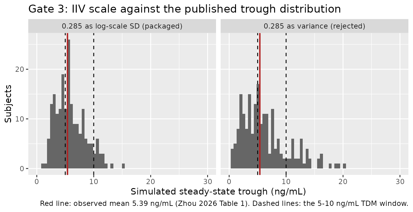
Gate 3 - published observed trough distribution, and the IIV scale
This is the gate that determines how the source’s
omegaCL/F = 0.285 must be read (see “Assumptions and
deviations”). Table S1 gives the number without saying whether it is the
log-scale SD or the NONMEM variance, and the two readings differ in
simulated spread by nearly a factor of two. Zhou 2026 Table 1 reports
the observed trough distribution as 5.39 +/- 2.31 ng/mL (CV
42.9%) over the 410 samples, which decides it.
ui_var <- ui |> rxode2::ini(etalcl = 0.285)   # the alternative reading
#> ℹ change initial estimate of `etalcl` to `0.285`

sim_pop_var <- solve_arm(ui_var, ev_pop, 101)

trough_of <- function(sim) {
  x <- sim$Cc[abs(sim$time - T_TROUGH) < 1e-8]
  stopifnot(length(x) == N_ARM)
  set.seed(4242)
  x <- x * (1 + rnorm(length(x), 0, 0.204))   # 20.4% proportional residual error
  x[x > 0]
}

t_sd  <- trough_of(sim_pop)
t_var <- trough_of(sim_pop_var)

summarise_trough <- function(x, label) {
  tibble::tibble(
    Reading = label,
    Median  = median(x),
    Mean    = mean(x),
    `CV (%)` = 100 * sd(x) / mean(x),
    `q10`   = quantile(x, 0.10),
    `q90`   = quantile(x, 0.90)
  )
}

dist_tab <- dplyr::bind_rows(
  tibble::tibble(Reading = "OBSERVED (Zhou 2026 Table 1)",
                 Median = NA_real_, Mean = 5.39, `CV (%)` = 100 * 2.31 / 5.39,
                 q10 = NA_real_, q90 = NA_real_),
  summarise_trough(t_sd,  "omega = 0.285 read as log-scale SD"),
  summarise_trough(t_var, "omega = 0.285 read as variance")
)
knitr::kable(dist_tab, digits = 2,
caption = "Gate 3: simulated steady-state trough distribution at the published median dose (3 mg/day q12h) under the two readings of omegaCL/F, against the observed distribution.")| Reading | Median | Mean | CV (%) | q10 | q90 |
|---|---|---|---|---|---|
| OBSERVED (Zhou 2026 Table 1) | NA | 5.39 | 42.86 | NA | NA |
| omega = 0.285 read as log-scale SD | 5.82 | 6.20 | 45.38 | 3.15 | 9.73 |
| omega = 0.285 read as variance | 5.90 | 7.00 | 71.63 | 2.22 | 13.16 |
The SD reading lands within a few percent of the observed spread; the variance reading overshoots it by roughly 70%. The simulation holds the dose at the published median while the observed figure additionally contains real dose variability (total daily dose IQR 3-4 mg), so a slight excess of simulated over observed CV is expected – but the variance reading would require the TDM loop to have removed about two thirds of the concentration variance, in a cohort where TDM control was demonstrably loose (46.6% of samples below the 5-10 ng/mL window). The assertions are on the centre and on robust quantiles, not on cohort extrema.
obs_cv <- 100 * 2.31 / 5.39
cv_sd  <- 100 * sd(t_sd)  / mean(t_sd)
cv_var <- 100 * sd(t_var) / mean(t_var)

stopifnot(
  # Structural: a mis-transcribed CL/F, V/F, dose or unit conversion moves the
  # whole distribution by tens of percent and blows this immediately.
  abs(median(t_sd) - 5.39) / 5.39 < 0.25,
  # The SD reading is consistent with the published spread (about 6% above it
  # at 1000 subjects; a 200-subject cohort once put it 15% above), and a CV
  # still carries ~2 points of sampling noise at this size, so the bound is
  # 1.25 -- far below the ~1.7 the variance reading produces ...
  cv_sd / obs_cv < 1.25,
  # ... and the variance reading is decisively rejected by it.
  cv_var / obs_cv > 1.5,
  # The two readings are separated by much more than Monte-Carlo noise.
  cv_var / cv_sd > 1.4
)
c(observed_CV = obs_cv, CV_sd_reading = cv_sd, CV_variance_reading = cv_var)
#>         observed_CV       CV_sd_reading CV_variance_reading
#>            42.85714            45.38462            71.63079
dplyr::bind_rows(
  tibble::tibble(Cc = t_sd,  Reading = "0.285 as log-scale SD (packaged)"),
  tibble::tibble(Cc = t_var, Reading = "0.285 as variance (rejected)")
) |>
  ggplot(aes(Cc)) +
  geom_histogram(bins = 40, fill = "grey40") +
  geom_vline(xintercept = c(5, 10), linetype = "dashed") +
  geom_vline(xintercept = 5.39, colour = "firebrick", linewidth = 0.8) +
  facet_wrap(~Reading) +
  coord_cartesian(xlim = c(0, 30)) +
  labs(
    x = "Simulated steady-state trough (ng/mL)", y = "Subjects",
    title = "Gate 3: IIV scale against the published trough distribution",
    caption = paste(
      "Red line: observed mean 5.39 ng/mL (Zhou 2026 Table 1).",
      "Dashed lines: the 5-10 ng/mL TDM window."
    )
  )
Gate 4 - PKNCA
Steady-state exposure over the final dosing interval, plus the
terminal half-life from the washout tail. The half-life is checked
against each subject’s own analytic value,
log(2) * (V/F) / (CL/F), computed from the
CL/F that subject actually drew.
sim_nca <- sim_pop |>
  dplyr::filter(!is.na(Cc)) |>
  dplyr::select(id, time, Cc, treatment)

# Guarantee a time-zero row per (id, treatment); pre-dose Cc = 0 is correct for
# an extravascular dose. Never filter on `time > 0` or `Cc > 0`.
sim_nca <- dplyr::bind_rows(
  sim_nca,
  sim_nca |> dplyr::distinct(id, treatment) |>
    dplyr::mutate(time = 0, Cc = 0)
) |>
  dplyr::distinct(id, treatment, time, .keep_all = TRUE) |>
  dplyr::arrange(id, treatment, time)

stopifnot(nrow(sim_nca) > 0, all(sim_nca$Cc >= 0))

conc_obj <- PKNCA::PKNCAconc(sim_nca, Cc ~ time | treatment + id)

dose_df <- ev_pop |>
  dplyr::filter(evid == 1) |>
  dplyr::select(id, time, amt, treatment)

dose_obj <- PKNCA::PKNCAdose(dose_df, amt ~ time | treatment + id)

intervals <- data.frame(
  start     = c(T_LAST,  T_TROUGH),
  end       = c(T_TROUGH, Inf),
  cmax      = c(TRUE,  FALSE),
  tmax      = c(TRUE,  FALSE),
  cmin      = c(TRUE,  FALSE),
  auclast   = c(TRUE,  FALSE),
  half.life = c(FALSE, TRUE)
)

nca_res <- PKNCA::pk.nca(PKNCA::PKNCAdata(conc_obj, dose_obj, intervals = intervals))
nca <- as.data.frame(nca_res)
stopifnot(nrow(nca) > 0)
# Take cmax / tmax / cmin / auclast from the dosing interval and half.life from
# the terminal interval. The interval filter is load-bearing, not cosmetic:
# PKNCA computes `tmax` for the terminal interval as well (it is a lambda.z
# dependency), so selecting on PPTESTCD alone leaves two `tmax` rows per
# subject and `pivot_wider()` then silently returns list-columns instead of
# erroring -- the failure only surfaces later, as "'x' must be atomic" inside
# an unrelated median().
nca_wide <- nca |>
  dplyr::filter(
    PPTESTCD %in% c("cmax", "tmax", "cmin", "auclast", "half.life"),
    (PPTESTCD == "half.life") == (start == T_TROUGH)
  ) |>
  dplyr::select(id, PPTESTCD, PPORRES) |>
  tidyr::pivot_wider(names_from = PPTESTCD, values_from = PPORRES)

# Fail loudly if a future PKNCA version emits another duplicate dependency:
# every column must be an atomic numeric of exactly one row per subject.
stopifnot(
  nrow(nca_wide) == N_ARM,
  all(vapply(nca_wide, is.numeric, logical(1)))
)

nca_wide |>
  dplyr::select(cmax, tmax, cmin, auclast, half.life) |>
  tidyr::pivot_longer(dplyr::everything(), names_to = "Parameter", values_to = "v") |>
  dplyr::group_by(Parameter) |>
  dplyr::summarise(
    Median = median(v, na.rm = TRUE),
    q05    = quantile(v, 0.05, na.rm = TRUE),
    q95    = quantile(v, 0.95, na.rm = TRUE),
    .groups = "drop"
  ) |>
  dplyr::rename("5th percentile" = q05, "95th percentile" = q95) |>
  knitr::kable(
    digits = 2,
    caption = "Gate 4: PKNCA steady-state exposure over the final 12 h dosing interval (cmax in ng/mL, tmax and half.life in h, auclast as AUCtau in ng*h/mL)."
)| Parameter | Median | 5th percentile | 95th percentile |
|---|---|---|---|
| auclast | 86.47 | 49.33 | 146.67 |
| cmax | 8.50 | 5.46 | 13.49 |
| cmin | 5.91 | 2.88 | 10.89 |
| half.life | 20.75 | 11.85 | 35.19 |
| tmax | 0.75 | 0.75 | 1.00 |
Zhou 2026 reports no NCA parameters, so there is no published table
to place alongside these; nlmixr2lib::ncaComparisonTable()
is therefore not used. The half-life is instead gated against the
model’s own analytic terminal rate.
Read tmax in that table as grid-quantised rather than
estimated: the dosing interval is observed on a 0.25 h grid, the
analytic peak for a typical subject is near 0.96 h, and the profile is
flat enough around the peak that every subject lands on the same 0.75 h
node. Nothing is asserted on it. cmin (the steady-state
trough, median 5.92 ng/mL) is the quantity comparable to the paper’s
observed 5.39 +/- 2.31 ng/mL, and it is Gate 3 that tests it.
analytic <- sim_pop |>
  dplyr::group_by(id) |>
  dplyr::summarise(t_half = log(2) * dplyr::first(vc) / dplyr::first(cl),
                   .groups = "drop")

hl <- nca_wide |>
  dplyr::select(id, half.life) |>
  dplyr::inner_join(analytic, by = "id") |>
  dplyr::filter(!is.na(half.life)) |>
  dplyr::mutate(pct_diff = 100 * (half.life - t_half) / t_half)

stopifnot(nrow(hl) == N_ARM)
c(n = nrow(hl),
  median_pct_diff = median(hl$pct_diff),
  max_abs_pct_diff = max(abs(hl$pct_diff)))
#>                n  median_pct_diff max_abs_pct_diff
#>     1.000000e+03     9.824051e-05     1.194866e+01

# Both sides use the same drawn CL/F, so the difference is regression and
# integrator error only; a tight bound is correct here.
stopifnot(
  abs(median(hl$pct_diff)) < 1,
  quantile(abs(hl$pct_diff), 0.95) < 2
)
The absorption half-life implied by the fixed ka of 4.5
1/h is 0.15 h, some two orders of magnitude faster than the terminal
half-life, so the model is firmly in the flip-flop-free regime and the
terminal phase is elimination-rate limited, as the authors assumed when
they fixed ka from the literature.
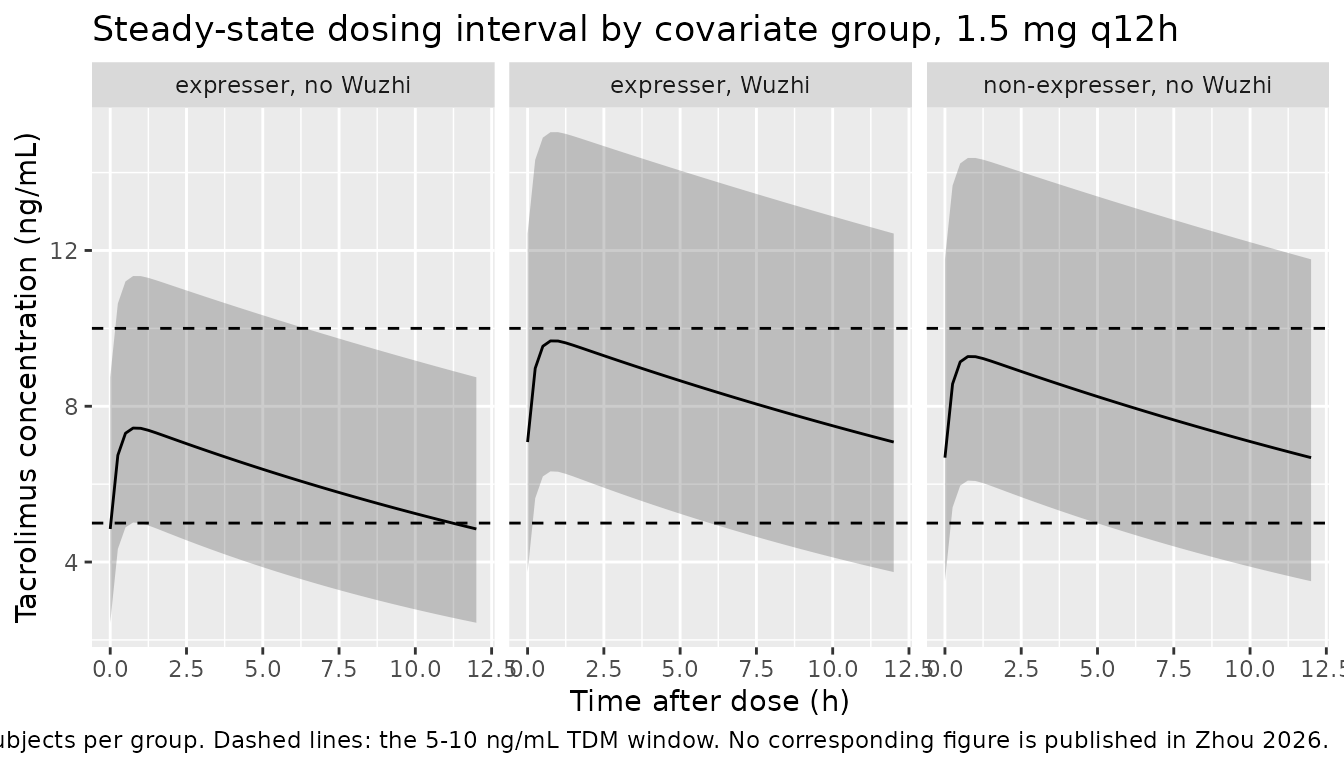
Steady-state profile by genotype
sim_cov |>
  dplyr::filter(time >= T_LAST, time <= T_TROUGH) |>
  dplyr::mutate(tad = time - T_LAST) |>
  dplyr::group_by(treatment, tad) |>
  dplyr::summarise(
    Q05 = quantile(Cc, 0.05), Q50 = quantile(Cc, 0.50),
    Q95 = quantile(Cc, 0.95), .groups = "drop"
  ) |>
  ggplot(aes(tad, Q50)) +
  geom_ribbon(aes(ymin = Q05, ymax = Q95), alpha = 0.25) +
  geom_line() +
  geom_hline(yintercept = c(5, 10), linetype = "dashed") +
  facet_wrap(~treatment) +
  labs(
    x = "Time after dose (h)", y = "Tacrolimus concentration (ng/mL)",
    title = "Steady-state dosing interval by covariate group, 1.5 mg q12h",
    caption = paste(
      "Median with 5th-95th percentile band, 200 subjects per group.",
      "Dashed lines: the 5-10 ng/mL TDM window. No corresponding figure is",
      "published in Zhou 2026."
    )
  )
Assumptions and deviations
-
The IIV scale is a determination, not a
transcription. Zhou 2026 Table S1 reports the row
omegaCL/Fas a bare0.285and the Results equation substitutes it directly into the exponential (... * e^0.285) where the eta belongs. Nothing in the paper says whether that number is the log-scale SD (omega) or the NONMEM variance (omega squared). It is encoded here as the log-scale SD, i.e.etalcl ~ 0.285^2 = 0.081225, on the following evidence:- Gate 3 above: the SD reading reproduces the observed trough CV of 42.9% (Table 1: 5.39 +/- 2.31 ng/mL) to within a few percent, while the variance reading overshoots it by roughly 70% and would require the TDM loop to have removed two thirds of the variance in a cohort where 46.6% of samples sat below the target window.
- The symbol omega, as distinct from omega squared, conventionally denotes the SD.
- The closest sibling model in this library,
Xiang_2025_tacrolimus- same journal, same drug, same two covariates, same one-compartment trough-only structure - reports IIV onCL/Fof 32.6% CV, against 29.1% here under the SD reading and 57.4% under the variance reading. Two tests that might have settled it do not, and were not relied on. The bootstrap-CI relative width,(0.33 - 0.23) / 0.282 = 0.355, falls between the SD prediction3.92 * sqrt(1 / (2 * 141)) = 0.233and the variance prediction3.92 * sqrt(2 / 141) = 0.467. The reported RSE of 17.1% sits nearer the variance asymptote, but omega RSEs estimated from sparse trough-only data routinely run two to three times above asymptotic values, so it carries little weight. A reviewer who prefers the variance reading can change one number inini(); Gate 3 will then fail, which is the intent.
-
The machine-learning half of the paper is out of
scope. The CatBoost / AdaBoost / GraBoost voting ensemble has
no ODE structure and its fitted coefficients are not published (it is
distributed only as a Streamlit application), so it cannot be
represented as an
rxode2model or reproduced from the paper. The individualCL/Fthat the ensemble consumes as its most influential feature is exactly what this model produces. -
Specimen matrix is internally inconsistent in the
source. Zhou 2026 calls the measurement “TAC plasma
concentration” throughout, but the assay described in Methods is the
Abbott ARCHITECT i1000sr with the ARCHITECT Tacrolimus Reagent Kit,
which is a whole-blood assay; tacrolimus partitions heavily into
erythrocytes and is universally monitored in whole blood, which is also
what the paper’s own 5-10 ng/mL target refers to.
compartmentDatarecords the specimen as whole blood withverified = FALSE. Nothing numerical depends on this:V/FandCL/Fare apparent parameters in whichever matrix was assayed. -
WZCis glossed incorrectly in the source. Results expands WZC as “compound Salvia miltiorrhiza polyphenolic acid capsule”. Wuzhi capsule is a Schisandra sphenanthera preparation, which is also what the paper’s own Discussion and its reference 27 describe (inhibition of CYP3A and P-glycoprotein). The canonical covariateCONMED_WUZHIis used, and the mis-gloss is recorded in itsnotes. -
CYP3A5 value inversion. Zhou 2026 codes the
*3/*3non-expresser as the affected group; the canonical register mandates the expresser-equals-1 orientation forCYP3A5_EXPRand explicitly instructs papers using a*3/*3indicator to record values under that name with the inversion documented. The published 0.768 is therefore applied as0.768^(1 - CYP3A5_EXPR). The direction of the effect is unchanged. -
theta_CL/FCin the displayed equation is read astheta_CL/F. The Results equation prints the leading term astheta_CL/FCwhereas Table S1 labels the rowthetaCL/F (L/h); the trailing “C” has no referent anywhere in the paper and is taken as a typesetting artefact of the equation image. -
Screened-but-unretained covariates. Body weight,
BMI, albumin, creatinine clearance, blood urea nitrogen, total
bilirubin, age and sex were collected and screened but not retained in
the population PK model; most were carried only into the
machine-learning feature set. They are documented in
covariatesDataExcludedrather thancovariateDataso that they do not register as declared-but-unused covariates. - Simulated dose is the published median. The cohorts use 1.5 mg q12h (total daily dose 3.00 mg, the Table 1 median). The real cohort’s doses ranged more widely (IQR 3.00-4.00 mg/day) and were TDM-titrated; the residual dose variability that this omits is the reason a small excess of simulated over observed CV is expected in Gate 3 even under the correct IIV scale.
- No published figure or NCA table to replicate. Zhou 2026’s Figure 2 is an NPDE diagnostic (which is by construction standard normal for the fitted model and so carries no information about the encoding), and Figures 3-6 belong to the machine-learning half. There is no published concentration-time profile, typical-value prediction or NCA table, so Gates 1, 2 and 4 validate the encoding against closed-form and internal-consistency targets and Gate 3 against the one published distributional anchor.
- Race and ethnicity are recorded but not simulated. The cohort is multi-ethnic (Han 67.1%, Kazakh or Uyghur 27.1%, Hui 4.6%, other 1.2%) and Zhou 2026 discusses inter-ethnic differences in CYP3A5 allele frequency at length, but ethnicity enters the model only through the genotype distribution, which the population arm reproduces directly.