Meropenem (Onichimowski 2020)
Source:vignettes/articles/Onichimowski_2020_meropenem.Rmd
Onichimowski_2020_meropenem.RmdModel and source
- Citation: Onichimowski D, Bedzkowska A, Ziolkowski H, Jaroszewski J, Borys M, Czuczwar M, Wiczling P. Population pharmacokinetics of standard-dose meropenem in critically ill patients on continuous renal replacement therapy: a prospective observational trial. Pharmacol Rep. 2020;72(3):719-729. doi:10.1007/s43440-020-00104-3
- Description: Two-compartment IV population PK model for meropenem in 19 critically ill adults on continuous renal replacement therapy (CVVH or CVVHD) receiving 1 g as a 1-h infusion q8h (Onichimowski 2020). Elimination is a single first-order clearance attributed to CRRT (ClCRRT); central volume V1 scales with serum albumin by a power function with exponent -2.87 around the 24.6 g/L cohort median. Log-normal IIV on V1, ClCRRT and V2 (IIV on Q fixed to zero); combined additive + proportional residual error.
- Article: https://doi.org/10.1007/s43440-020-00104-3 (open access)
Population
Onichimowski et al. ran a prospective, single-centre observational study in a tertiary medical/surgical ICU in Olsztyn, Poland. Twenty critically ill adults on continuous renal replacement therapy (CRRT) were enrolled and 19 contributed PK data (5 female, 14 male; age 36-79 years, median 67; body weight 60-100 kg, median 80). Nine patients were on CVVH with heparin anticoagulation and ten on CVVHD with regional citrate anticoagulation, all with an AV 1000 polysulfone 1.8 m^2 filter. Ten were septic. Median serum albumin was 24.6 g/L (range 15.6-31.8), median APACHE II 31 and median SOFA 10 (Table 1). Every patient received meropenem 1 g as a 1-h infusion every 8 h. Arterial samples were taken before the dose and at 15, 30, 45, 60, 75, 90, 120, 180, 240 and 480 min after the start of the infusion, giving 256 concentrations.
Source trace
| Element | Value | Source location |
|---|---|---|
| Structure | Two compartments, IV infusion, elimination from central (ClCRRT) | Methods Eq. 1-2; ADVAN3 TRANS4 |
lvc |
V1 = 27.9 L at ALB = 24.6 g/L | Table 2 |
lcl |
ClCRRT = 15.1 L/h | Table 2 |
lq |
Q = 21.1 L/h | Table 2 |
lvp |
V2 = 33.7 L | Table 2 |
e_alb_vc |
-2.87 (power on ALB / 24.6) | Table 2; Results equation
V1,i = 27.9 (ALB_i/24.6)^-2.87 exp(eta)
|
etalvc |
53.1 %CV -> omega^2 = log(0.531^2 + 1) = 0.248 | Table 2 and footnote |
etalcl |
43.7 %CV -> 0.175 | Table 2 and footnote |
etalvp |
85.6 %CV -> 0.550 | Table 2 and footnote |
| IIV on Q | 0, fixed (omitted) | Table 2; Results text |
addSd |
0.881 mg/L | Table 2 |
propSd |
24.1 %CV -> 0.241 | Table 2; Methods Eq. 4 |
Model
mod <- readModelDb("Onichimowski_2020_meropenem")
mod_ui <- rxode2::rxode(mod)
#> ℹ parameter labels from comments will be replaced by 'label()'
mod_typ <- rxode2::zeroRe(mod_ui)
V1 against albumin (Figure 2, upper panel)
alb_grid <- data.frame(ALB = seq(15, 32, by = 0.5)) |>
  mutate(V1 = 27.9 * (ALB / 24.6)^-2.87)
ggplot(alb_grid, aes(ALB, V1)) +
  geom_line() +
  labs(x = "Albumin (g/L)", y = "Typical V1 (L)",
       title = "Replicates Figure 2 (upper panel) of Onichimowski 2020")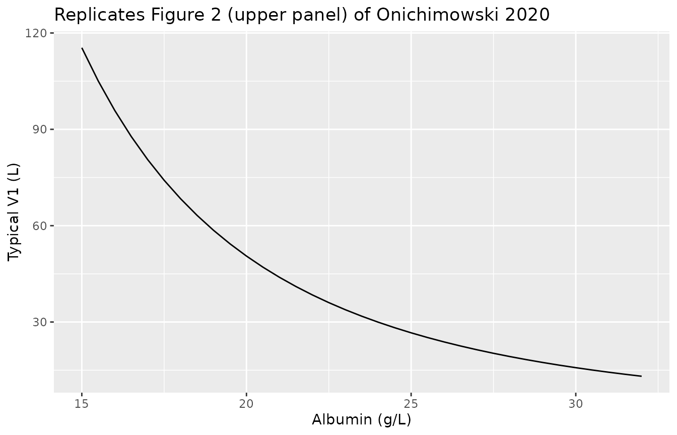
Typical first-dose and steady-state profiles
alb_levels <- c(15.6, 24.6, 31.8)
ev_typ <- rxode2::et(amt = 1000, dur = 1, ii = 8, addl = 29, cmt = "central") |>
  rxode2::et(c(seq(0, 8, by = 0.05), seq(232, 240, by = 0.05)), cmt = "central") |>
  as.data.frame()
typ <- bind_rows(lapply(alb_levels, function(a) {
  d <- ev_typ
  d$ALB <- a
  s <- as.data.frame(rxode2::rxSolve(mod_typ, d, returnType = "data.frame"))
  s$ALB <- a
  s
}))
#> ℹ omega/sigma items treated as zero: 'etalvc', 'etalcl', 'etalvp'
#> ℹ omega/sigma items treated as zero: 'etalvc', 'etalcl', 'etalvp'
#> ℹ omega/sigma items treated as zero: 'etalvc', 'etalcl', 'etalvp'
typ |>
  mutate(
    period = ifelse(time <= 8, "First dose", "Steady state (dose 30)"),
    tad = ifelse(time <= 8, time, time - 232)
  ) |>
  ggplot(aes(tad, Cc, colour = factor(ALB))) +
  geom_line() +
  facet_wrap(~period) +
  scale_y_log10() +
  labs(x = "Time after start of infusion (h)", y = "Meropenem (mg/L)",
       colour = "Albumin (g/L)",
       title = "Typical profiles, 1 g as a 1-h infusion q8h")
#> Warning in scale_y_log10(): log-10 transformation introduced infinite values.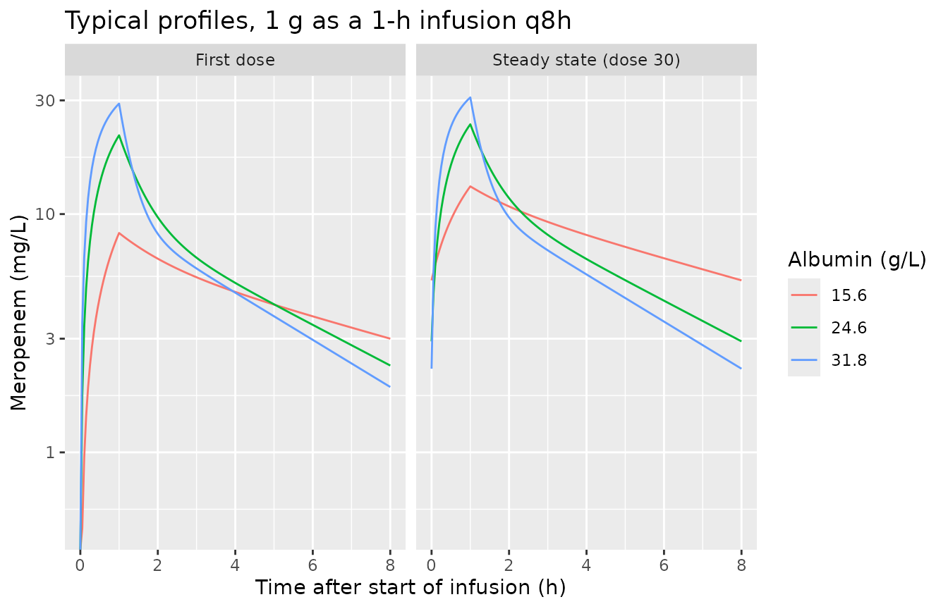
The observed first-dose concentrations in Figure 1 of the paper peak at roughly 20-60 mg/L and fall to about 2-10 mg/L at 8 h, consistent with the typical curves above.
Probability of target attainment (Figure 4)
The paper simulated 1000 subjects at steady state after 1 g as a 1-h infusion q8h for albumin 15.6, 24.6 and 31.8 g/L and counted the fraction reaching 40% and 100% T > MIC over 24 h. Here 200 virtual subjects per albumin level are simulated with between-subject variability on the final estimates; the last 24 h of a 30-dose course is used as steady state.
rxode2::rxSetSeed(20200416)
n_per_arm <- 200
obs_ss <- seq(216, 240, by = 0.1)
ev_pta <- bind_rows(lapply(seq_along(alb_levels), function(i) {
  e <- rxode2::et(amt = 1000, dur = 1, ii = 8, addl = 29, cmt = "central") |>
    rxode2::et(obs_ss, cmt = "central") |>
    rxode2::et(id = seq_len(n_per_arm) + (i - 1) * n_per_arm) |>
    as.data.frame()
  e$ALB <- alb_levels[i]
  e
}))
sim_pta <- as.data.frame(rxode2::rxSolve(mod_ui, ev_pta, keep = "ALB",
                                         returnType = "data.frame"))
ft_mic <- function(sim, mic) {
  sim |>
    filter(time >= 216) |>
    group_by(ALB, id) |>
    summarise(ft = mean(Cc > mic), .groups = "drop")
}
mics <- 2^seq(-4, 6, by = 0.5)
pta <- bind_rows(lapply(mics, function(m) {
  ft_mic(sim_pta, m) |>
    group_by(ALB) |>
    summarise(pta40 = mean(ft >= 0.4), pta100 = mean(ft >= 1), .groups = "drop") |>
    mutate(MIC = m)
}))
pta |>
  pivot_longer(c(pta40, pta100), names_to = "target", values_to = "PTA") |>
  mutate(target = ifelse(target == "pta40", "40% T > MIC", "100% T > MIC")) |>
  ggplot(aes(MIC, PTA * 100, colour = factor(ALB))) +
  geom_line() +
  geom_hline(yintercept = 90, linetype = "dashed") +
  scale_x_log10() +
  facet_wrap(~target) +
  labs(x = "MIC (mg/L)", y = "PTA (%)", colour = "Albumin (g/L)",
       title = "Replicates Figure 4a and 4c of Onichimowski 2020")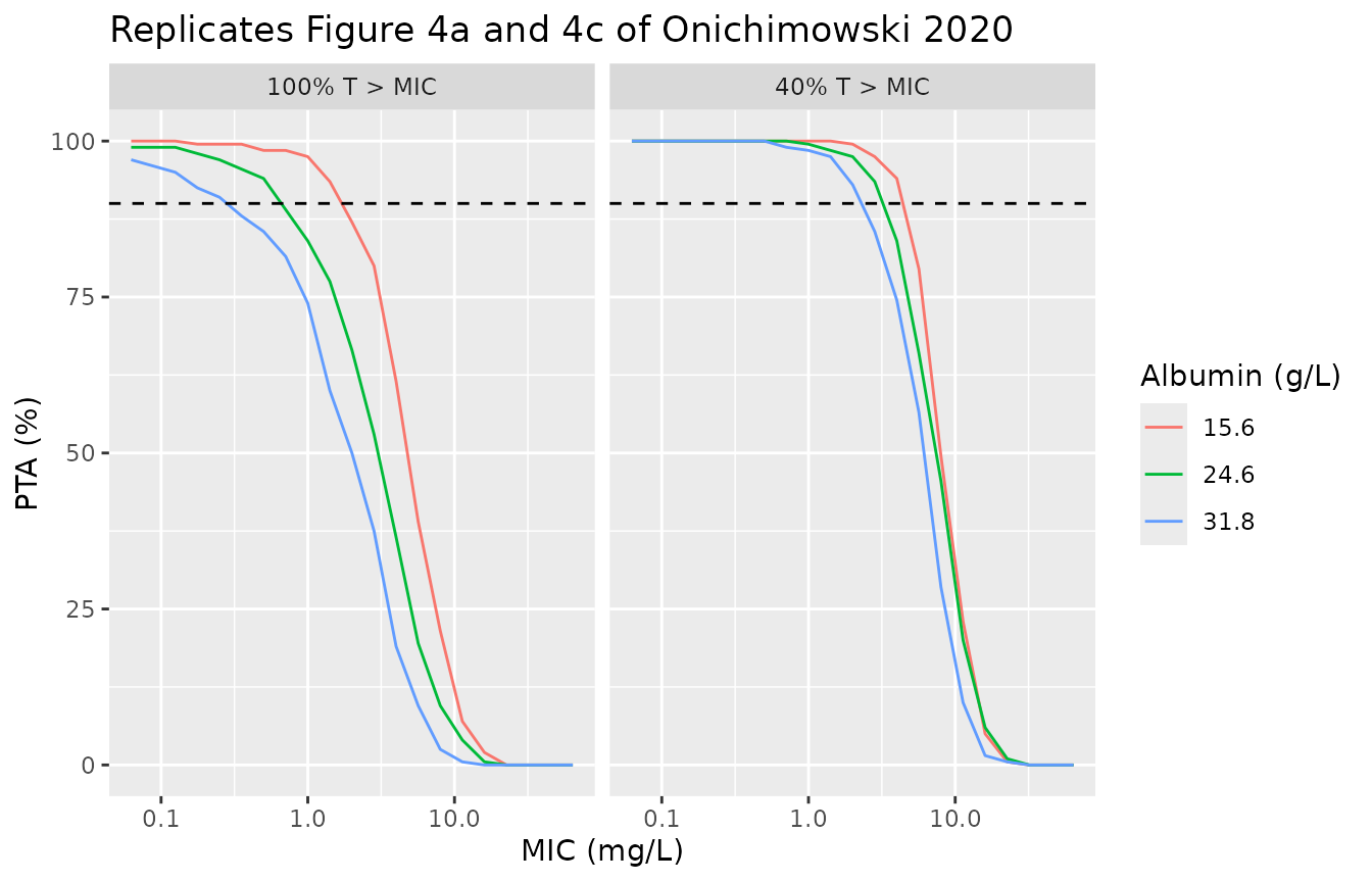
pta2 <- ft_mic(sim_pta, 2) |>
  group_by(ALB) |>
  summarise(pta40 = 100 * mean(ft >= 0.4), pta100 = 100 * mean(ft >= 1), .groups = "drop") |>
  mutate(
    pub40 = c(99.8, 97.8, 95.3),
    pub100 = c(91.8, 70.0, 58.7)
  )
pta2 |>
  select(ALB, pta40, pub40, pta100, pub100) |>
  dplyr::rename(
    "Albumin (g/L)" = ALB,
    "Simulated PTA 40% T>2 mg/L (%)" = pta40,
    "Published PTA 40% T>2 mg/L (%)" = pub40,
    "Simulated PTA 100% T>2 mg/L (%)" = pta100,
    "Published PTA 100% T>2 mg/L (%)" = pub100
  ) |>
knitr::kable(digits = 1)| Albumin (g/L) | Simulated PTA 40% T>2 mg/L (%) | Published PTA 40% T>2 mg/L (%) | Simulated PTA 100% T>2 mg/L (%) | Published PTA 100% T>2 mg/L (%) |
|---|---|---|---|---|
| 15.6 | 99.5 | 99.8 | 87.0 | 91.8 |
| 24.6 | 97.5 | 97.8 | 66.5 | 70.0 |
| 31.8 | 93.0 | 95.3 | 50.0 | 58.7 |
The 40% target is reached by nearly every subject at all three albumin levels, and the 100% target falls with rising albumin, as in the paper. The published PTA values are bootstrap medians that fold parameter uncertainty in on top of between-subject variability, and each simulated arm here has 200 subjects (Monte Carlo SE about 3 percentage points at 70%), so agreement is checked with a band rather than exactly.
PKNCA validation
The paper reports no NCA. As an internal check, PKNCA is run on the typical (no-variability) steady-state interval at each albumin level; at steady state AUC over one dosing interval must equal dose / CL = 1000 / 15.1 = 66.2 mg*h/L regardless of albumin, because albumin acts only on V1.
nca_in <- typ |>
  filter(time >= 232, !is.na(Cc)) |>
  mutate(id = match(ALB, alb_levels), treatment = paste0("ALB ", ALB, " g/L"))
dose_df <- nca_in |>
  distinct(id, treatment) |>
  mutate(time = 232, amt = 1000)
conc_obj <- PKNCA::PKNCAconc(nca_in, Cc ~ time | treatment + id)
dose_obj <- PKNCA::PKNCAdose(dose_df, amt ~ time | treatment + id)
intervals <- data.frame(start = 232, end = 240, cmax = TRUE, tmax = TRUE,
                        cmin = TRUE, auclast = TRUE)
nca_res <- PKNCA::pk.nca(PKNCA::PKNCAdata(conc_obj, dose_obj, intervals = intervals))
nca_tab <- as.data.frame(nca_res) |>
  select(treatment, PPTESTCD, PPORRES) |>
  pivot_wider(names_from = PPTESTCD, values_from = PPORRES)
nca_tab |>
  dplyr::rename(
    "Group" = treatment,
    "Cmax (mg/L)" = cmax,
    "Tmax (h)" = tmax,
    "Cmin (mg/L)" = cmin,
    "AUC0-8,ss (mg*h/L)" = auclast
  ) |>
knitr::kable(digits = 2)| Group | AUC0-8,ss (mg*h/L) | Cmax (mg/L) | Cmin (mg/L) | Tmax (h) |
|---|---|---|---|---|
| ALB 15.6 g/L | 66.22 | 13.07 | 5.27 | 1 |
| ALB 24.6 g/L | 66.22 | 23.81 | 2.92 | 1 |
| ALB 31.8 g/L | 66.22 | 30.87 | 2.24 | 1 |
Assumptions and deviations
- IIV on Q was fixed to zero by the authors because it tended to zero;
it is omitted from
ini()rather than carried as a zero-variance eta. - Table 2 gives IIV as %CV with the footnote
%CV = sqrt(exp(IIV^2 - 1) * 100%; the misplaced parenthesis is read as the standard log-normal conversionCV = sqrt(exp(omega^2) - 1), soomega^2 = log(CV^2 + 1). - The proportional residual error is reported as “sigma^2 prop, %CV = 24.1” and is encoded as a proportional SD of 0.241; the additive term (0.881 mg/L) is taken as an SD.
- The model has a single elimination clearance, which the authors label ClCRRT; no residual renal or non-renal clearance was separated from it, and CRRT settings were not retained as covariates.
- The simulated PTA uses the point estimates only; the paper’s values also integrate bootstrap parameter uncertainty, so their confidence intervals are wider than the between-subject variability alone produces.