Albinterferon alfa-2b population PK and SVR exposure-response (Riggs 2012)
Source:vignettes/articles/Riggs_2012_albinterferon.Rmd
Riggs_2012_albinterferon.Rmd
library(nlmixr2lib)
library(rxode2)
#> rxode2 5.1.8 using 2 threads (see ?getRxThreads)
#>   no cache: create with `rxCreateCache()`
library(PKNCA)
#>
#> Attaching package: 'PKNCA'
#> The following object is masked from 'package:stats':
#>
#>     filter
library(dplyr)
#>
#> Attaching package: 'dplyr'
#> The following objects are masked from 'package:stats':
#>
#>     filter, lag
#> The following objects are masked from 'package:base':
#>
#>     intersect, setdiff, setequal, union
library(ggplot2)
Riggs et al. (2012), J Clin Pharmacol 52(4):475-486, doi:10.1177/0091270011399576, report three separate models for albinterferon alfa-2b (albIFN), a genetic fusion of recombinant human albumin with recombinant interferon alfa-2b developed for chronic hepatitis C virus (HCV) infection:
- a one-compartment population PK model with first-order absorption, fitted in NONMEM VI to 12,042 serum concentrations from 1984 patients;
- a logistic regression for sustained virologic response (SVR) in the
HCV genotype 1 subpopulation, fitted with
glmin R; and - the same logistic regression fitted separately to the genotype 2/3 subpopulation.
Because the authors fitted the two SVR analyses independently on disjoint subpopulations, they are carried as two model files rather than as one model with a genotype term.
pk   <- rxode2::rxode(readModelDb("Riggs_2012_albinterferon"))
svr1 <- rxode2::rxode(readModelDb("Riggs_2012_albinterferon_svr_gt1"))
svr23 <- rxode2::rxode(readModelDb("Riggs_2012_albinterferon_svr_gt23"))
Population
pop <- pk$population
tibble::tibble(
  Field = names(pop),
  Value = vapply(pop, function(x) paste(
    if (is.null(names(x))) as.character(x) else paste0(names(x), " ", x),
    collapse = ", "), character(1))
) |>
knitr::kable(caption = "Population metadata for the Riggs 2012 population PK analysis set.")| Field | Value |
|---|---|
| species | human |
| n_subjects | 1984 |
| n_studies | 5 |
| age_range | 18-79 years |
| weight_range | 38-166 kg |
| sex_female_pct | 40.1 |
| race_ethnicity | White 81, Asian 13, Black 5, Other 1 |
| disease_state | Chronic hepatitis C virus infection with detectable serum HCV RNA and compensated liver disease. 66% HCV genotype 1, the remainder genotype 2 or 3 apart from 5 patients with genotype 4. Interferon-treatment-naive except for one phase 2 trial (NCT00097435), which enrolled patients who had failed previous interferon alfa treatment. |
| dose_range | 900-1800 ug albinterferon alfa-2b, self-administered subcutaneously in the thigh or abdomen once every 2 weeks or once every 4 weeks, for 48 weeks (genotype 1) or 24 weeks (genotype 2/3); up to 72 weeks for late responders in NCT00097435. All patients also received daily oral ribavirin per the standard of care for their genotype. The 1200 ug every-2-weeks arms of the phase 3 trials were reduced to 900 ug during the studies because of serious pulmonary adverse events. |
| regions | multinational |
| notes | Pooled from three phase 2 and two phase 3 randomized trials (NCT00656006, NCT00097435, NCT00115908, NCT00411385, NCT00402428), contributing 12,042 serum albIFN concentrations. Full baseline demographics are in Supplementary Table I, which was not available when this model was built; the figures given here are those stated in the main-text Results, ‘Population PK Analysis’. sex_female_pct is computed from the reported counts (795 women of 1984). Serum albIFN was measured by ELISA with a lower limit of quantitation of 0.53 ng/mL for all phase 3 specimens and most phase 2 specimens, and 0.26 ng/mL for the remainder. Hypothetical reference individual for the Table I estimates: 45-year-old white woman, 75 kg, HCV genotype 1, negative for immunogenicity, baseline HCV RNA < 800,000 IU/mL, ribavirin 1200 mg/day, abdomen as injection site, albumin 4.3 g/dL, ALT 34 IU/L, estimated creatinine clearance 120 mL/min. |
The analysis pooled three phase 2 and two phase 3 randomised trials (NCT00656006, NCT00097435, NCT00115908, NCT00411385, NCT00402428). Patients self-administered albIFN subcutaneously into the thigh or abdomen every 2 or 4 weeks, for 48 weeks (genotype 1) or 24 weeks (genotype 2/3), together with daily oral ribavirin. The phase 3 1200 ug every-2-weeks arms were reduced to 900 ug mid-study after the data-monitoring committee flagged serious pulmonary adverse events.
The exposure-response analyses used the 1869 interferon-naive patients that remain after excluding trial NCT00097435, which enrolled prior interferon non-responders.
Source trace
Every value in the three model files, and where it came from. The paper’s displayed structural equations sit on p. 479; the parameter table is Table I (pp. 476-477) and the SVR table is Table II (p. 482).
tibble::tribble(
  ~Quantity, ~`Source location`, ~Note,
  "CL/F, V/F, ka typical values", "Table I, row 'None'", "38.9 mL/h, 11.6 L, 0.0148 1/h; converted to L/h and L in the model file",
  "CL/F covariate equation", "p. 479, displayed equation 1", "theta4, 5, 10, 11, 12 power exponents; theta6-9, 13-16, 18, 42, 43 multiplicative",
  "V/F covariate equation", "p. 479, displayed equation 2", "theta19, 20, 25 power exponents; theta21-24, 26-29 multiplicative",
  "ka covariate equation", "p. 479, displayed equation 3", "theta39 (weight) and theta30 (age) exponents; theta31-38, 40 multiplicative",
  "Bioavailability switch", "p. 479, 'F1 = 1; if injection site = thigh, then F1 = theta44'", "theta44 = 1.07 from Table I, row 'Frel for thigh as injection site'",
  "Covariate normalisations", "p. 479, 'where' block", "TWT = WT/75 kg, TAGE = AGE/45 y, TALB = ALB/4.3, TALT = ALT/34, TCRL = min(CRCL,150)/120, TRIB = tabs per day / 6",
  "Covariate coefficient values", "Table I, all rows", "point estimates; bootstrap medians and 95% CIs recorded in the ini() comments",
  "Reference individual", "Table I footnote b", "45 y white woman, 75 kg, genotype 1, immunogenicity negative, HCV RNA < 800,000 IU/mL, RBV 1200 mg/d, abdomen, ALB 4.3 g/dL, ALT 34 IU/L, CrCl 120 mL/min",
  "IIV (CV%) on CL/F, V/F, ka", "Results p. 480", "21%, 34%, 24%; converted with omega^2 = log(CV^2 + 1)",
  "CL/F-V/F covariance", "Results p. 480", "reported only as 'minimal'; no numeric value published (entered as 0)",
  "Residual error", "Results p. 480", "proportional CV 27%, additive SD 1.51 ng/mL",
  "SVR model form", "Methods p. 478", "logistic regression via glm, separately per genotype stratum",
  "SVR coefficients", "Table II (both columns)", "recovered by logit inversion of the tabulated probabilities; see 'SVR exposure-response' below",
  "SVR reference individual", "Table II footnote a and Figure 2 caption", "48 wk (GT1) or 24 wk (GT2/3), Cavg 75 ng/mL, HCV RNA 400,000-800,000 IU/mL, white or other race, weight < 75 kg, no dose reduction"
) |>
knitr::kable(caption = "Source trace for the Riggs 2012 extraction.")| Quantity | Source location | Note |
|---|---|---|
| CL/F, V/F, ka typical values | Table I, row ‘None’ | 38.9 mL/h, 11.6 L, 0.0148 1/h; converted to L/h and L in the model file |
| CL/F covariate equation | p. 479, displayed equation 1 | theta4, 5, 10, 11, 12 power exponents; theta6-9, 13-16, 18, 42, 43 multiplicative |
| V/F covariate equation | p. 479, displayed equation 2 | theta19, 20, 25 power exponents; theta21-24, 26-29 multiplicative |
| ka covariate equation | p. 479, displayed equation 3 | theta39 (weight) and theta30 (age) exponents; theta31-38, 40 multiplicative |
| Bioavailability switch | p. 479, ‘F1 = 1; if injection site = thigh, then F1 = theta44’ | theta44 = 1.07 from Table I, row ‘Frel for thigh as injection site’ |
| Covariate normalisations | p. 479, ‘where’ block | TWT = WT/75 kg, TAGE = AGE/45 y, TALB = ALB/4.3, TALT = ALT/34, TCRL = min(CRCL,150)/120, TRIB = tabs per day / 6 |
| Covariate coefficient values | Table I, all rows | point estimates; bootstrap medians and 95% CIs recorded in the ini() comments |
| Reference individual | Table I footnote b | 45 y white woman, 75 kg, genotype 1, immunogenicity negative, HCV RNA < 800,000 IU/mL, RBV 1200 mg/d, abdomen, ALB 4.3 g/dL, ALT 34 IU/L, CrCl 120 mL/min |
| IIV (CV%) on CL/F, V/F, ka | Results p. 480 | 21%, 34%, 24%; converted with omega^2 = log(CV^2 + 1) |
| CL/F-V/F covariance | Results p. 480 | reported only as ‘minimal’; no numeric value published (entered as 0) |
| Residual error | Results p. 480 | proportional CV 27%, additive SD 1.51 ng/mL |
| SVR model form | Methods p. 478 | logistic regression via glm, separately per genotype stratum |
| SVR coefficients | Table II (both columns) | recovered by logit inversion of the tabulated probabilities; see ‘SVR exposure-response’ below |
| SVR reference individual | Table II footnote a and Figure 2 caption | 48 wk (GT1) or 24 wk (GT2/3), Cavg 75 ng/mL, HCV RNA 400,000-800,000 IU/mL, white or other race, weight < 75 kg, no dose reduction |
Typical-value replication
These checks are deterministic: one typical subject, inter-individual variability zeroed, covariates set to the Table I footnote b reference individual. They validate the transcription of the structural parameters and of the covariate equations against quantities the paper states in prose, and are asserted tightly because there is no cohort sampling involved.
tau <- 24 * 14  # every 2 weeks, in hours

# Table I footnote b reference individual. ALB is supplied in SI g/L
# (4.3 g/dL = 43 g/L); CRCL is raw mL/min, not BSA-normalised.
ref_cov <- function(wt = 75, injsite_thigh = 0) {
  data.frame(
    WT = wt, AGE = 45, ALB = 43, ALT = 34, CRCL = 120, SEXF = 1,
    RACE_ASIAN = 0, RACE_BLACK = 0, RACE_OTHER = 0,
    HCV_GT2 = 0, HCV_GT3 = 0, HCV_GT4 = 0,
    HCV_VLOAD = 5e5, DOSE_RBV_MGD = 1200, ADA_POS = 0,
    CONMED_CYP2D6_INH = 0, CONMED_CYP3A4_INH = 0,
    INJSITE_THIGH = injsite_thigh
  )
}

pk_typ <- rxode2::zeroRe(pk)

solve_typical <- function(dose, wt = 75, injsite_thigh = 0, n_dose = 12, by = 2) {
  ev <- rxode2::et(amt = dose, ii = tau, until = tau * (n_dose - 1), cmt = "depot") |>
    rxode2::et(seq(0, tau * n_dose, by = by), cmt = "central")
  cov <- ref_cov(wt, injsite_thigh)
  cov$id <- 1L
  out <- as.data.frame(rxode2::rxSolve(pk_typ, ev, cov, addDosing = FALSE,
                                       returnType = "data.frame"))
  if (is.null(out$id)) out$id <- 1L
  out
}

typ <- solve_typical(900)
#> ℹ omega/sigma items treated as zero: 'etalcl', 'etalvc', 'etalka'
cl_typ <- mean(typ$cl)
vc_typ <- mean(typ$vc)
ka_typ <- mean(typ$ka)
thalf_typ <- log(2) * vc_typ / cl_typ
tibble::tribble(
  ~Quantity,                       ~Published,  ~Model,
  "CL/F (mL/h)",                   38.9,        round(cl_typ * 1000, 2),
  "V/F (L)",                       11.6,        round(vc_typ, 3),
  "ka (1/h)",                      0.0148,      round(ka_typ, 5),
  "Terminal half-life (h)",        200,         round(thalf_typ, 1)
) |>
knitr::kable(caption = "Typical-value parameters for the Table I reference individual. The published half-life is the paper's own 'approximately 200 hours' derived from CL/F and V/F (Results p. 480).")| Quantity | Published | Model |
|---|---|---|
| CL/F (mL/h) | 38.9000 | 38.9000 |
| V/F (L) | 11.6000 | 11.6000 |
| ka (1/h) | 0.0148 | 0.0148 |
| Terminal half-life (h) | 200.0000 | 206.7000 |
stopifnot(
  abs(cl_typ * 1000 - 38.9) < 1e-6,
  abs(vc_typ - 11.6) < 1e-6,
  abs(ka_typ - 0.0148) < 1e-9,
  # The paper's own rounding of log(2) * 11.6 / 0.0389 = 206.7 h.
  abs(thalf_typ - 206.7) < 0.1
)
Average steady-state concentration against its closed form
For a linear one-compartment model the average concentration over a
steady-state dosing interval is exactly Dose / (CL * tau),
independent of absorption. Both sides here use the same parameters, so
this is a pure numerical-integration check and is asserted tightly.
cavg_ss <- function(s) {
  last <- s[s$time >= max(s$time) - tau, ]
  mean(last$Cc)  # uniform 2 h grid: the mean is the trapezoidal average
}
auc_first <- function(s) mean(s$Cc[s$time <= tau])

cavg_tbl <- lapply(c(900, 1200), function(d) {
  s <- solve_typical(d)
  tibble::tibble(
    `Dose (ug q2wk)` = d,
    # Dose is in ug and vc in L, so Dose / (CL * tau) is ug/L = ng/mL with
    # no further scaling -- the same identity the model relies on for Cc.
    `Closed form Dose/(CL*tau)` = round(d / (cl_typ * tau), 2),
    `Simulated Cavg,ss` = round(cavg_ss(s), 2)
  )
}) |> dplyr::bind_rows()
#> ℹ omega/sigma items treated as zero: 'etalcl', 'etalvc', 'etalka'
#> ℹ omega/sigma items treated as zero: 'etalcl', 'etalvc', 'etalka'

knitr::kable(cavg_tbl, caption = "Simulated steady-state average concentration (ng/mL) against its closed form.")| Dose (ug q2wk) | Closed form Dose/(CL*tau) | Simulated Cavg,ss |
|---|---|---|
| 900 | 68.86 | 68.73 |
| 1200 | 91.81 | 91.64 |
Accumulation
The paper states that “accumulation of albIFN in serum was about 40% for the q2wk dosing regimens, calculated from the individual estimates as the ratio of AUC during a dosing interval for the first dose and at steady state” (Results p. 480).
Read literally, the quantity named is
AUC(first interval) / AUC(steady-state interval), and
“about 40%” is one minus that ratio – i.e. the share of steady-state
exposure attributable to accumulation. That reading reproduces the
published number from the transcribed CL/F and V/F. The alternative
reading, the fold-increase AUC_ss / AUC_first - 1, would be
about 72% and does not match. Both are computed below so the arithmetic
is explicit.
s900 <- solve_typical(900)
#> ℹ omega/sigma items treated as zero: 'etalcl', 'etalvc', 'etalka'
r_first_over_ss <- auc_first(s900) / cavg_ss(s900)

tibble::tribble(
  ~Quantity, ~Value,
  "AUC(first interval) / AUC(steady-state interval)", round(r_first_over_ss, 4),
  "1 - that ratio (matches the published 'about 40%')", round(1 - r_first_over_ss, 4),
  "AUC_ss / AUC_first - 1 (the alternative reading)",  round(1 / r_first_over_ss - 1, 4)
) |>
knitr::kable(caption = "Accumulation, both readings of the published sentence.")| Quantity | Value |
|---|---|
| AUC(first interval) / AUC(steady-state interval) | 0.5820 |
| 1 - that ratio (matches the published ‘about 40%’) | 0.4180 |
| AUC_ss / AUC_first - 1 (the alternative reading) | 0.7183 |
The weight-exposure relationship
The single covariate finding the authors regarded as clinically meaningful. Results p. 481 states that steady-state exposure would increase approximately 2-fold for a typical 50 kg patient compared with a typical 125 kg patient, and that relative to the 75 kg reference there would be an exposure increase of about 30% at 50 kg and decreases of 20% and 30% at 100 and 125 kg. This is an exact, deterministic gate on the weight exponent for CL/F.
base_cavg <- cavg_ss(solve_typical(900, wt = 75))
#> ℹ omega/sigma items treated as zero: 'etalcl', 'etalvc', 'etalka'
wt_tbl <- tibble::tibble(
  `Weight (kg)` = c(50, 100, 125),
  Published = c("+30%", "-20%", "-30%"),
  Model = sprintf("%+.0f%%", 100 * (vapply(c(50, 100, 125),
    function(w) cavg_ss(solve_typical(900, wt = w)), numeric(1)) / base_cavg - 1))
)
#> ℹ omega/sigma items treated as zero: 'etalcl', 'etalvc', 'etalka'
#> ℹ omega/sigma items treated as zero: 'etalcl', 'etalvc', 'etalka'
#> ℹ omega/sigma items treated as zero: 'etalcl', 'etalvc', 'etalka'
knitr::kable(wt_tbl, caption = "Change in steady-state exposure relative to the 75 kg reference individual.")| Weight (kg) | Published | Model |
|---|---|---|
| 50 | +30% | +32% |
| 100 | -20% | -18% |
| 125 | -30% | -30% |
ratio_50_125 <- cavg_ss(solve_typical(900, wt = 50)) / cavg_ss(solve_typical(900, wt = 125))
#> ℹ omega/sigma items treated as zero: 'etalcl', 'etalvc', 'etalka'
#> ℹ omega/sigma items treated as zero: 'etalcl', 'etalvc', 'etalka'
cat(sprintf("50 kg vs 125 kg exposure ratio: %.2f (published: approximately 2-fold)\n", ratio_50_125))
#> 50 kg vs 125 kg exposure ratio: 1.87 (published: approximately 2-fold)

stopifnot(
  abs(cavg_ss(solve_typical(900, wt = 50))  / base_cavg - 1.30) < 0.05,
  abs(cavg_ss(solve_typical(900, wt = 100)) / base_cavg - 0.80) < 0.05,
  abs(cavg_ss(solve_typical(900, wt = 125)) / base_cavg - 0.70) < 0.05,
  abs(ratio_50_125 - 2) < 0.15
)
#> ℹ omega/sigma items treated as zero: 'etalcl', 'etalvc', 'etalka'
#> ℹ omega/sigma items treated as zero: 'etalcl', 'etalvc', 'etalka'
#> ℹ omega/sigma items treated as zero: 'etalcl', 'etalvc', 'etalka'
Injection site
Thigh injection carries both a 1.09 multiplicative effect on
ka and a relative bioavailability of 1.07 versus the
abdomen. Because steady-state exposure depends on bioavailability but
not on absorption rate, the thigh / abdomen exposure ratio must recover
theta44 = 1.07 exactly.
site_ratio <- cavg_ss(solve_typical(900, injsite_thigh = 1)) / base_cavg
#> ℹ omega/sigma items treated as zero: 'etalcl', 'etalvc', 'etalka'
ka_ratio <- mean(solve_typical(900, injsite_thigh = 1)$ka) / ka_typ
#> ℹ omega/sigma items treated as zero: 'etalcl', 'etalvc', 'etalka'
cat(sprintf("Thigh / abdomen steady-state exposure ratio: %.4f (theta44 = 1.07)\n", site_ratio))
#> Thigh / abdomen steady-state exposure ratio: 1.0699 (theta44 = 1.07)
cat(sprintf("Thigh / abdomen ka ratio:                    %.4f (theta40 = 1.09)\n", ka_ratio))
#> Thigh / abdomen ka ratio:                    1.0900 (theta40 = 1.09)
stopifnot(abs(site_ratio - 1.07) < 0.002, abs(ka_ratio - 1.09) < 1e-6)
Virtual cohort
The original data are not public and the paper’s baseline-demographics table (Supplementary Table I) is not available, so the covariate distributions below are assumed, constrained to the ranges and proportions the main-text Results do state (1984 patients, 795 women, ages 18-79 years, weights 38-166 kg, 81% White / 13% Asian / 5% Black, 66% genotype 1). Everything not stated in the main text – the shape of the weight distribution, the baseline HCV-RNA, ALT, albumin and creatinine-clearance distributions, immunogenicity and comedication rates – is an illustrative choice and is listed under Assumptions and deviations below.
This is why the tight validation gates in this vignette are the deterministic ones above; the cohort comparisons that follow are consistency checks whose agreement depends on demographics we cannot verify.
The two phase 3 regimens are simulated on the same
200 virtual subjects, with the random-number seed reset before each arm
so that every subject draws identical CL/F,
V/F and ka random effects in both. Common
random numbers make the between-regimen comparison a paired one, which
turns dose proportionality into an exact per-subject check rather than a
noisy between-cohort one.
set.seed(20120401)
n_sub <- 200L

# Truncated draws helper: resample until inside [lo, hi].
rtrunc <- function(n, rfun, lo, hi) {
  x <- rfun(n)
  bad <- which(x < lo | x > hi)
  while (length(bad)) {
    x[bad] <- rfun(length(bad))
    bad <- which(x < lo | x > hi)
  }
  x
}

wt <- rtrunc(n_sub, function(k) rlnorm(k, log(82), 0.22), 38, 166)
# Race: 81 / 13 / 5 / 1 per cent White / Asian / Black / Other.
race <- sample(c("White", "Asian", "Black", "Other"), n_sub,
               replace = TRUE, prob = c(0.81, 0.13, 0.05, 0.01))
# Genotype: 66% GT1, remainder split between GT2 and GT3. Genotype 4 is
# omitted: only 5 of 1984 patients carried it, and the model file flags
# simulations at HCV_GT4 = 1 as extrapolation rather than estimation.
gt <- sample(c(1, 2, 3), n_sub, replace = TRUE, prob = c(0.66, 0.17, 0.17))

cohort <- data.frame(
  id = seq_len(n_sub),
  WT = wt,
  AGE = rtrunc(n_sub, function(k) rnorm(k, 47, 9), 18, 79),
  ALB = rtrunc(n_sub, function(k) rnorm(k, 43, 3.5), 30, 55),
  ALT = rtrunc(n_sub, function(k) rlnorm(k, log(60), 0.6), 10, 400),
  CRCL = rtrunc(n_sub, function(k) rnorm(k, 110, 25), 40, 200),
  SEXF = rbinom(n_sub, 1, 795 / 1984),
  RACE_ASIAN = as.integer(race == "Asian"),
  RACE_BLACK = as.integer(race == "Black"),
  RACE_OTHER = as.integer(race == "Other"),
  HCV_GT2 = as.integer(gt == 2),
  HCV_GT3 = as.integer(gt == 3),
  HCV_GT4 = 0L,
  HCV_VLOAD = rlnorm(n_sub, log(1.2e6), 1.1),
  # Standard weight-banded adult ribavirin dosing.
  DOSE_RBV_MGD = ifelse(wt < 75, 1000, 1200),
  ADA_POS = rbinom(n_sub, 1, 0.05),
  CONMED_CYP2D6_INH = rbinom(n_sub, 1, 0.05),
  CONMED_CYP3A4_INH = rbinom(n_sub, 1, 0.05),
  INJSITE_THIGH = rbinom(n_sub, 1, 0.5)
)
stopifnot(!anyDuplicated(cohort$id))

# Descriptive labels are kept OUT of the covariate frame: rxSolve coerces the
# whole parameter frame to numeric and errors on character columns.
labels_df <- data.frame(
  id = cohort$id,
  weight_band = ifelse(cohort$WT < 75, "< 75 kg", ">= 75 kg"),
  sex = ifelse(cohort$SEXF == 1, "Women", "Men"),
  genotype = ifelse(gt == 1, "Genotype 1", "Genotype 2/3")
)

tibble::tibble(
  n = n_sub,
  `Median weight (kg)` = round(median(cohort$WT), 1),
  `Weight range (kg)` = sprintf("%.0f-%.0f", min(cohort$WT), max(cohort$WT)),
  `Median age (y)` = round(median(cohort$AGE), 0),
  `Women (%)` = round(100 * mean(cohort$SEXF), 1),
  `Genotype 1 (%)` = round(100 * mean(gt == 1), 1)
) |>
knitr::kable(caption = "Simulated virtual cohort (assumed covariate distributions).")| n | Median weight (kg) | Weight range (kg) | Median age (y) | Women (%) | Genotype 1 (%) |
|---|---|---|---|---|---|
| 200 | 82.2 | 43-147 | 48 | 44 | 63.5 |
n_dose <- 10L  # 20 weeks; with a 207 h half-life this is well past steady state
obs_grid <- seq(0, tau * n_dose, by = 8)

solve_arm <- function(dose) {
  # Reset the seed INSIDE the loop so both arms draw the same random effects.
  rxode2::rxSetSeed(20120401)
  ev <- rxode2::et(amt = dose, ii = tau, until = tau * (n_dose - 1), cmt = "depot") |>
    rxode2::et(obs_grid, cmt = "central") |>
    rxode2::et(id = cohort$id)
  out <- as.data.frame(rxode2::rxSolve(pk, ev, cohort,
                                       addDosing = FALSE, returnType = "data.frame"))
  out$treatment <- paste0(dose, " ug q2wk")
  out$dose <- dose
  out
}

sim <- dplyr::bind_rows(solve_arm(900), solve_arm(1200)) |>
  dplyr::left_join(labels_df, by = "id")

stopifnot(nrow(sim) > 0, !anyNA(sim$Cc), all(sim$Cc >= 0), !anyNA(sim$weight_band))
Common random numbers make dose proportionality exact per subject:
the individual CL/F values are identical between arms, so
each subject’s steady-state exposure must scale by exactly 1200/900. Any
departure is numerical error alone, so this is asserted at machine
precision.
cavg_sub <- sim |>
  dplyr::filter(time >= tau * (n_dose - 1)) |>
  dplyr::group_by(treatment, id) |>
  dplyr::summarise(cav = mean(Cc), cl = mean(cl), .groups = "drop")

wide <- cavg_sub |>
  tidyr::pivot_wider(id_cols = id, names_from = treatment,
                     values_from = c(cav, cl))

cl_dev <- max(abs(wide$`cl_1200 ug q2wk` / wide$`cl_900 ug q2wk` - 1))
ratio_dev <- max(abs(wide$`cav_1200 ug q2wk` / wide$`cav_900 ug q2wk` - 1200 / 900))
cat(sprintf("max |CL(1200)/CL(900) - 1|      = %.3g\n", cl_dev))
#> max |CL(1200)/CL(900) - 1|      = 0
cat(sprintf("max |Cavg ratio - 1200/900|     = %.3g\n", ratio_dev))
#> max |Cavg ratio - 1200/900|     = 8.13e-12

stopifnot(nrow(wide) == n_sub, cl_dev < 1e-12, ratio_dev < 1e-10)
sim |>
  dplyr::group_by(treatment, time) |>
  dplyr::summarise(med = median(Cc), lo = quantile(Cc, 0.05),
                   hi = quantile(Cc, 0.95), .groups = "drop") |>
  ggplot(aes(time / 24 / 7, med, ymin = lo, ymax = hi, fill = treatment, colour = treatment)) +
  geom_ribbon(alpha = 0.2, colour = NA) +
  geom_line() +
  labs(x = "Time (weeks)", y = "Serum albIFN (ng/mL)",
       colour = "Regimen", fill = "Regimen") +
  theme_bw()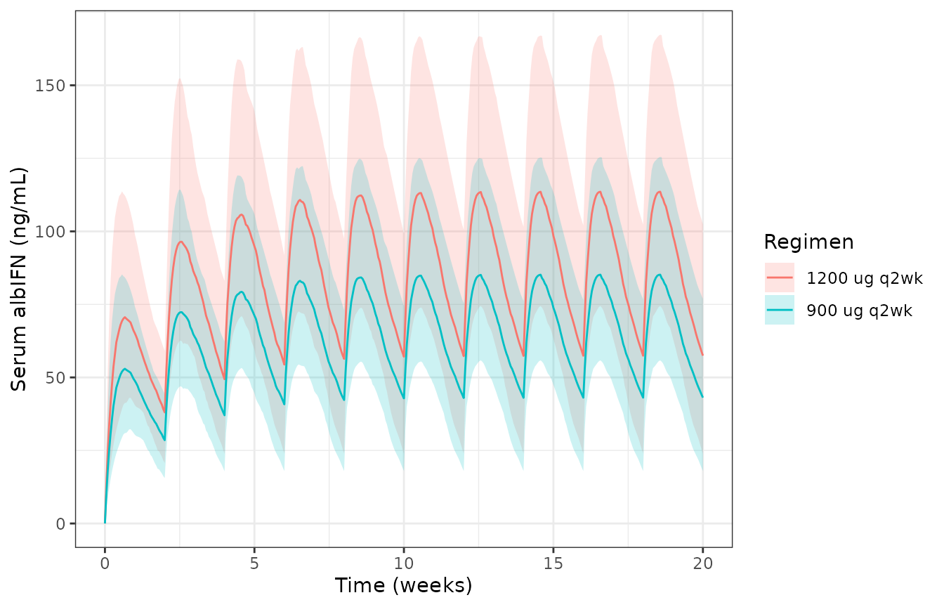
Simulated albinterferon serum concentration-time profiles over ten every-2-weeks doses. Lines are the median and the 5th-95th percentiles across the virtual cohort.
NCA validation with PKNCA
sim_nca <- sim |>
  dplyr::filter(!is.na(Cc)) |>
  dplyr::select(id, time, Cc, treatment)

# Defensive time-zero record (extravascular: pre-dose concentration is 0).
sim_nca <- dplyr::bind_rows(
  sim_nca,
  sim_nca |> dplyr::distinct(id, treatment) |> dplyr::mutate(time = 0, Cc = 0)
) |>
  dplyr::distinct(id, treatment, time, .keep_all = TRUE) |>
  dplyr::arrange(id, treatment, time)

dose_df <- sim |>
  dplyr::distinct(id, treatment, amt = dose) |>
  tidyr::crossing(time = seq(0, tau * (n_dose - 1), by = tau)) |>
  dplyr::select(id, time, amt, treatment)
stopifnot(nrow(dose_df) == 2L * n_sub * n_dose)

conc_obj <- PKNCA::PKNCAconc(sim_nca, Cc ~ time | treatment + id,
                             concu = "ng/mL", timeu = "h")
dose_obj <- PKNCA::PKNCAdose(dose_df, amt ~ time | treatment + id,
                             doseu = "ug")

start_ss <- tau * (n_dose - 1)
intervals <- data.frame(
  start   = c(0, start_ss),
  end     = c(tau, start_ss + tau),
  # Disjoint parameter sets so each PPTESTCD appears exactly once per subject:
  # Cmax and Tmax characterise the FIRST dose (which is what the paper's Cmax
  # is), while Cav and Cmin characterise the STEADY-STATE interval.
  cmax    = c(TRUE, FALSE),
  tmax    = c(TRUE, FALSE),
  cav     = c(FALSE, TRUE),
  cmin    = c(FALSE, TRUE)
)

nca_res <- PKNCA::pk.nca(PKNCA::PKNCAdata(conc_obj, dose_obj, intervals = intervals))
Comparison against the published exposure summary
Riggs 2012 (Results p. 480) reports, for the two every-2-weeks
regimens, the mean of the individual Cmax
estimates following the first dose and the mean of the
individual Cavg estimates. Cavg is the paper’s
average steady-state concentration; Cav is PKNCA’s name for
the same quantity over the steady-state interval.
published <- tibble::tribble(
  ~treatment,       ~cmax, ~cav,
  "900 ug q2wk",    56.6,  66.2,
  "1200 ug q2wk",   76.2,  86.4
)

cmp <- nlmixr2lib::ncaComparisonTable(
  simulated     = nca_res,
  reference     = published,
  by            = "treatment",
  params        = c("cmax", "cav"),
  units         = c(cmax = "ng/mL", cav = "ng/mL"),
  tolerance_pct = 20
)

knitr::kable(cmp, caption = "Simulated versus published albIFN exposure. * differs from the reference by more than 20%.")| NCA parameter | treatment | Reference | Simulated | % diff |
|---|---|---|---|---|
| Cmax (ng/mL) | 900 ug q2wk | 56.6 | 55.8 | -1.5% |
| Cmax (ng/mL) | 1200 ug q2wk | 76.2 | 74.4 | -2.4% |
| Cavg (ng/mL) | 900 ug q2wk | 66.2 | 66.8 | +1.0% |
| Cavg (ng/mL) | 1200 ug q2wk | 86.4 | 89.1 | +3.2% |
attr(cmp, "footnote")
#> NULL
The steady-state Cav rows agree closely. The first-dose
Cmax rows sit below the published means, and there are two
reasons that are worth separating:
- The paper’s
Cmaxis a noncompartmental statistic taken from observed concentrations (Methods p. 478), so it is the maximum of a handful of measurements each carrying a 27% proportional residual error. The maximum of several noisy draws is biased upward relative to the underlying peak, and the albIFN profile is extremely flat around its peak (absorption half-life 47 h against an elimination half-life of 207 h), which puts many samples near the maximum and makes the bias larger. The simulated values here are individual model predictions, which carry no residual error. -
Cavis an integral and averages residual error away, which is exactly why it is unaffected.
The chunk below quantifies the first point rather than asserting it: it adds the paper’s own residual-error model to the simulated profiles and recomputes the observed maximum on a realistic sampling schedule. No parameter is changed.
prop_sd <- 0.27
add_sd  <- 1.51

# A plausible first-interval sampling schedule: weekly plus a mid-week sample.
sched <- c(0, 24, 72, 168, 240, 336)
first_int <- sim |>
  dplyr::filter(time %in% sched) |>
  dplyr::select(id, treatment, time, Cc)

set.seed(99)
obs_max <- first_int |>
  dplyr::mutate(Cobs = pmax(0, Cc * (1 + rnorm(dplyr::n(), 0, prop_sd)) +
                              rnorm(dplyr::n(), 0, add_sd))) |>
  dplyr::group_by(treatment, id) |>
  dplyr::summarise(pred_max = max(Cc), obs_max = max(Cobs), .groups = "drop") |>
  dplyr::group_by(treatment) |>
  dplyr::summarise(`Mean predicted max` = round(mean(pred_max), 1),
                   `Mean observed max` = round(mean(obs_max), 1),
                   `Inflation` = sprintf("%+.0f%%", 100 * (mean(obs_max) / mean(pred_max) - 1)),
                   .groups = "drop")
knitr::kable(obs_max, caption = "Effect of the published residual-error model on an observed-maximum Cmax, on a weekly-plus sampling schedule over the first dosing interval.")| treatment | Mean predicted max | Mean observed max | Inflation |
|---|---|---|---|
| 1200 ug q2wk | 75.7 | 85.3 | +13% |
| 900 ug q2wk | 56.8 | 63.0 | +11% |
cav_rows <- cmp[grepl("Cav", cmp[[1]], fixed = TRUE), ]
pct <- suppressWarnings(as.numeric(gsub("[^0-9.+-]", "", cav_rows$`% diff`)))
stopifnot(length(pct) == 2L, !anyNA(pct), all(abs(pct) < 15))
Cohort findings reported in the paper
Three further statements in Results p. 481 are cohort-level rather than typical-value, so they are checked on medians rather than on extremes.
cavg_by_subject <- as.data.frame(nca_res$result) |>
  dplyr::filter(PPTESTCD == "cav") |>
  dplyr::select(treatment, id, cav = PPORRES) |>
  dplyr::left_join(labels_df, by = "id")
stopifnot(nrow(cavg_by_subject) == 2L * n_sub, !anyNA(cavg_by_subject$weight_band))

wt_contrast <- cavg_by_subject |>
  dplyr::group_by(weight_band) |>
  dplyr::summarise(med = median(cav), .groups = "drop")
wt_pct <- 100 * (wt_contrast$med[wt_contrast$weight_band == "< 75 kg"] /
                 wt_contrast$med[wt_contrast$weight_band == ">= 75 kg"] - 1)

sex_contrast <- cavg_by_subject |>
  dplyr::group_by(sex) |>
  dplyr::summarise(med = median(cav), .groups = "drop")
sex_pct <- 100 * (sex_contrast$med[sex_contrast$sex == "Women"] /
                  sex_contrast$med[sex_contrast$sex == "Men"] - 1)

# The model's OWN direct sex effect, isolated from any weight difference:
# the same reference individual solved as a woman and as a man. This is a
# deterministic counterfactual, so it recovers theta6 = 1.05 exactly.
cov_f <- ref_cov(); cov_f$id <- 1L
cov_m <- ref_cov(); cov_m$SEXF <- 0; cov_m$id <- 1L
ev1 <- rxode2::et(amt = 900, ii = tau, until = tau * 11, cmt = "depot") |>
  rxode2::et(seq(0, tau * 12, by = 2), cmt = "central")
cl_f <- mean(as.data.frame(rxode2::rxSolve(pk_typ, ev1, cov_f, addDosing = FALSE,
                                           returnType = "data.frame"))$cl)
#> ℹ omega/sigma items treated as zero: 'etalcl', 'etalvc', 'etalka'
cl_m <- mean(as.data.frame(rxode2::rxSolve(pk_typ, ev1, cov_m, addDosing = FALSE,
                                           returnType = "data.frame"))$cl)
#> ℹ omega/sigma items treated as zero: 'etalcl', 'etalvc', 'etalka'
direct_sex_pct <- 100 * (cl_m / cl_f - 1)

tibble::tribble(
  ~Statement, ~Published, ~Model,
  "Cavg in patients < 75 kg versus >= 75 kg (cohort)", "25% to 30% greater", sprintf("%+.0f%%", wt_pct),
  "Cavg in women versus men (cohort)",                 "approximately 25% greater", sprintf("%+.0f%%", sex_pct),
  "Direct model effect of male sex on CL/F",           "1.05 (Table I)", sprintf("%+.1f%%", direct_sex_pct)
) |>
knitr::kable(caption = "Cohort-level exposure contrasts, and the model's own direct sex effect isolated from body weight.")| Statement | Published | Model |
|---|---|---|
| Cavg in patients < 75 kg versus >= 75 kg (cohort) | 25% to 30% greater | +31% |
| Cavg in women versus men (cohort) | approximately 25% greater | +1% |
| Direct model effect of male sex on CL/F | 1.05 (Table I) | +5.0% |
stopifnot(
  # Weight band: a real, large, model-driven contrast that the cohort reproduces.
  wt_pct > 10,
  # Direct sex effect: deterministic, so recovered exactly.
  abs(direct_sex_pct - 5.0) < 0.01
)
The weight-band contrast reproduces the paper. The sex
contrast deliberately does not, and the table shows why. Riggs
2012 is explicit that sex “did not lend any additional description to PK
variability” when entered into the popPK model, and that women
nonetheless had roughly 25% greater Cavg because,
on average, men in this chronic HCV population weighed more than
women (Results p. 481). The model’s own direct sex effect is
only the 5% shown in the last row.
The virtual cohort draws body weight independently of sex, so it deliberately lacks the sex-weight correlation that produces the published 25%, and the cohort sex contrast is therefore reported without an assertion – it is dominated by sampling noise around that 5% direct effect. Building the correlation in would require a male/female weight gap the paper never quantifies, and asserting on the result would be asserting on an assumption. The assertion above is placed on the deterministic quantity instead, which is what actually validates the transcription of theta6.
SVR exposure-response
Riggs 2012 reports the SVR logistic regressions as Table II: a fitted SVR probability with a 95% confidence interval for a defined reference individual (“None”) and for ten one-covariate-at-a-time perturbations of it. The logit-scale coefficients are never printed.
Because every row perturbs exactly one covariate away from one common
reference, each coefficient is recovered exactly as a difference of
logits, and the intercept is the logit of the reference probability. The
recovery is self-validating: the intercept implied by
the two Cavg rows, extrapolated back to the reference
exposure of 75 ng/mL, agrees with the intercept read directly off the
“None” row to 0.001 (genotype 1) and 0.0001 (genotype 2/3) on the logit
scale. That agreement simultaneously confirms that Cavg
enters linearly on the logit scale – which the Methods leave open a
priori, allowing either a near-linear or a sigmoidal form – and that the
rows really are single-covariate perturbations of a shared
reference.
The round trip below re-derives all twenty published probabilities from the model files.
tab2 <- tibble::tribble(
  ~row,                         ~gt1,  ~gt23,
  "None",                       61.9,  82.8,
  "Reduced treatment duration", 14.8,  26.1,
  "Cavg 60 ng/mL",              59.6,  80.6,
  "Cavg 90 ng/mL",              64.1,  84.8,
  "HCV RNA < 400 000 IU/mL",    84.6,  96.9,
  "HCV RNA >= 800 000 IU/mL",   63.0,  82.7,
  "Asian race",                 73.9,  77.7,
  "Black race",                 42.4,  83.4,
  "Weight >= 75 kg",            59.8,  74.0,
  "Dose was reduced",           62.9,  86.4
)

# Table II footnote a / Figure 2 caption reference individual, perturbed one
# covariate at a time in the order of the table rows above.
svr_covariates <- function(full_weeks) {
  d <- data.frame(
    CSS_ALBIFN = rep(75, 10), T_TRT = full_weeks, HCV_VLOAD = 6e5,
    RACE_ASIAN = 0, RACE_BLACK = 0, WT = 70, DOSE_REDUCED = 0
  )
  d$T_TRT[2]         <- full_weeks / 2   # footnote b: 24 wk (GT1), 12 wk (GT2/3)
  d$CSS_ALBIFN[3]    <- 60
  d$CSS_ALBIFN[4]    <- 90
  d$HCV_VLOAD[5]     <- 3e5
  d$HCV_VLOAD[6]     <- 9e5
  d$RACE_ASIAN[7]    <- 1
  d$RACE_BLACK[8]    <- 1
  d$WT[9]            <- 80
  d$DOSE_REDUCED[10] <- 1
  d$id <- seq_len(10)
  d
}

svr_predict <- function(ui, full_weeks) {
  ev <- rxode2::et(0) |> rxode2::et(id = seq_len(10))
  out <- as.data.frame(rxode2::rxSolve(ui, ev, svr_covariates(full_weeks),
                                       addDosing = FALSE, returnType = "data.frame"))
  100 * out$psvr[order(out$id)]
}

svr_tbl <- tab2 |>
  dplyr::mutate(
    `GT1 model`  = round(svr_predict(svr1, 48), 1),
    `GT2/3 model` = round(svr_predict(svr23, 24), 1)
  ) |>
  dplyr::rename(`Covariate setting` = row,
                `GT1 published` = gt1,
                `GT2/3 published` = gt23) |>
  dplyr::select(`Covariate setting`, `GT1 published`, `GT1 model`,
                `GT2/3 published`, `GT2/3 model`)

knitr::kable(svr_tbl, caption = "Round trip of Riggs 2012 Table II: published SVR probabilities (%) against the model files.")| Covariate setting | GT1 published | GT1 model | GT2/3 published | GT2/3 model |
|---|---|---|---|---|
| None | 61.9 | 61.9 | 82.8 | 82.8 |
| Reduced treatment duration | 14.8 | 14.8 | 26.1 | 26.1 |
| Cavg 60 ng/mL | 59.6 | 59.6 | 80.6 | 80.6 |
| Cavg 90 ng/mL | 64.1 | 64.1 | 84.8 | 84.8 |
| HCV RNA < 400 000 IU/mL | 84.6 | 84.6 | 96.9 | 96.9 |
| HCV RNA >= 800 000 IU/mL | 63.0 | 63.0 | 82.7 | 82.7 |
| Asian race | 73.9 | 73.9 | 77.7 | 77.7 |
| Black race | 42.4 | 42.4 | 83.4 | 83.4 |
| Weight >= 75 kg | 59.8 | 59.8 | 74.0 | 74.0 |
| Dose was reduced | 62.9 | 62.9 | 86.4 | 86.4 |
stopifnot(
  nrow(svr_tbl) == 10L,
  max(abs(svr_tbl$`GT1 model`   - svr_tbl$`GT1 published`))   < 0.05,
  max(abs(svr_tbl$`GT2/3 model` - svr_tbl$`GT2/3 published`)) < 0.05
)
The exposure-response relationship itself
The paper’s central negative finding: across the studied exposure
range SVR is nearly flat in Cavg, and the two phase 3
regimens sit close together on it.
cavg_grid <- seq(20, 180, by = 2)
curve_cov <- function(full_weeks) {
  data.frame(
    id = seq_along(cavg_grid), CSS_ALBIFN = cavg_grid, T_TRT = full_weeks,
    HCV_VLOAD = 6e5, RACE_ASIAN = 0, RACE_BLACK = 0, WT = 70, DOSE_REDUCED = 0
  )
}
curve_for <- function(ui, full_weeks, label) {
  ev <- rxode2::et(0) |> rxode2::et(id = seq_along(cavg_grid))
  out <- as.data.frame(rxode2::rxSolve(ui, ev, curve_cov(full_weeks),
                                       addDosing = FALSE, returnType = "data.frame"))
  out <- out[order(out$id), ]
  data.frame(cavg = cavg_grid, psvr = out$psvr, stratum = label)
}

svr_curve <- dplyr::bind_rows(
  curve_for(svr1, 48, "Genotype 1"),
  curve_for(svr23, 24, "Genotype 2/3")
)

ggplot(svr_curve, aes(cavg, 100 * psvr, colour = stratum)) +
  geom_vline(xintercept = c(62.7, 83.0), linetype = "dashed", colour = "grey50") +
  geom_line(linewidth = 0.9) +
  coord_cartesian(ylim = c(0, 100)) +
  labs(x = "Average steady-state albIFN concentration (ng/mL)",
       y = "Predicted SVR probability (%)", colour = "Stratum") +
  theme_bw()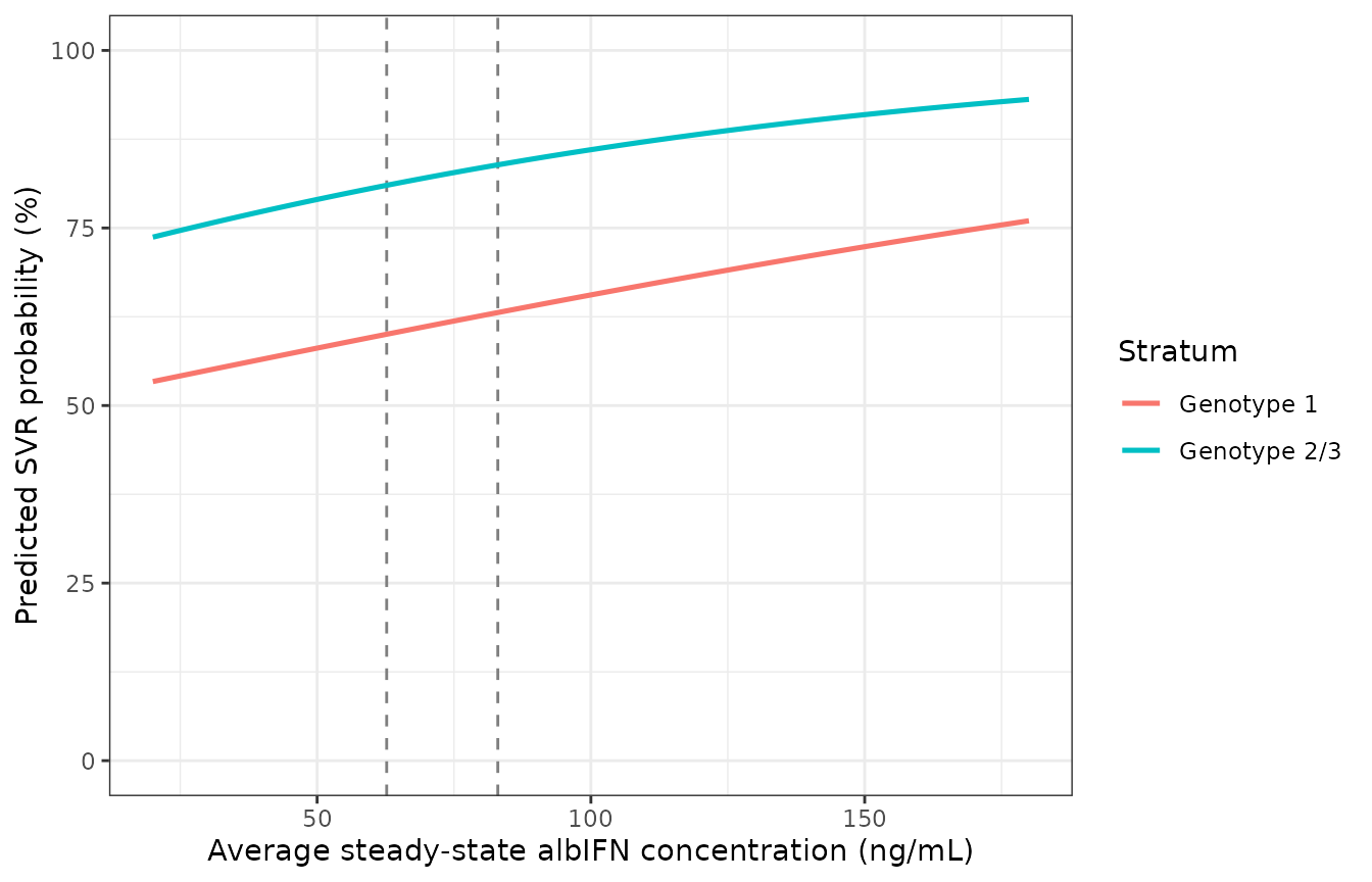
Predicted SVR probability against average steady-state albinterferon concentration for the reference individual in each genotype stratum. Vertical lines mark the published medians of the individual Cavg estimates for the 900 and 1200 ug every-2-weeks regimens (62.7 and 83.0 ng/mL).
span_rows <- svr_curve |> dplyr::filter(cavg >= 62.7, cavg <= 83.0)
# Guard: an empty filter would make the all() below vacuously TRUE.
stopifnot(nrow(span_rows) > 0, dplyr::n_distinct(span_rows$stratum) == 2L)

flat <- span_rows |>
  dplyr::group_by(stratum) |>
  dplyr::summarise(span_pct_points = 100 * (max(psvr) - min(psvr)), .groups = "drop")
stopifnot(nrow(flat) == 2L)

flat |>
  dplyr::rename(Stratum = stratum,
                `SVR change (percentage points)` = span_pct_points) |>
  knitr::kable(digits = 2,
caption = "Change in predicted SVR probability across the span between the two regimens' published median Cavg values (62.7 to 83.0 ng/mL).")| Stratum | SVR change (percentage points) |
|---|---|
| Genotype 1 | 2.71 |
| Genotype 2/3 | 2.55 |
Which predictors actually matter
ranked <- svr_tbl |>
  dplyr::filter(`Covariate setting` != "None") |>
  dplyr::mutate(
    `GT1 shift` = `GT1 model` - svr_tbl$`GT1 model`[svr_tbl$`Covariate setting` == "None"],
    `GT2/3 shift` = `GT2/3 model` - svr_tbl$`GT2/3 model`[svr_tbl$`Covariate setting` == "None"]
  ) |>
  dplyr::select(`Covariate setting`, `GT1 shift`, `GT2/3 shift`) |>
  dplyr::arrange(dplyr::desc(abs(`GT1 shift`)))
knitr::kable(ranked, digits = 1,
caption = "Change in SVR probability (percentage points) from the reference individual, ranked by the genotype 1 effect.")| Covariate setting | GT1 shift | GT2/3 shift |
|---|---|---|
| Reduced treatment duration | -47.1 | -56.7 |
| HCV RNA < 400 000 IU/mL | 22.7 | 14.1 |
| Black race | -19.5 | 0.6 |
| Asian race | 12.0 | -5.1 |
| Cavg 60 ng/mL | -2.3 | -2.2 |
| Cavg 90 ng/mL | 2.2 | 2.0 |
| Weight >= 75 kg | -2.1 | -8.8 |
| HCV RNA >= 800 000 IU/mL | 1.1 | -0.1 |
| Dose was reduced | 1.0 | 3.6 |
This reproduces the paper’s summary: reduced treatment duration and baseline HCV RNA dominate; Black race is a large negative effect in genotype 1 only; and both the exposure perturbations and the dose-reduction indicator are small. Riggs 2012 emphasises that the lower SVR rate in Black patients with genotype 1 appeared independent of any difference in albIFN exposure. Note that the genotype 2/3 Black-race estimate is essentially null but very imprecise (published 95% CI 45.6% to 96.8%), so the contrast between the strata should not be over-read.
Assumptions and deviations
Model structure and parameters
- CL/F-V/F covariance is entered as 0. The paper states a covariance term between the CL/F and V/F random effects was estimated but reports it only as “minimal” (Results p. 480), with no numeric value anywhere. The block OMEGA structure is preserved with the off-diagonal set to 0. Simulations that depend on the joint CL/F-V/F distribution will be slightly mis-specified; marginal distributions are unaffected.
-
IIV back-transform. The paper reports
interindividual variability as coefficients of variation (21%, 34%,
24%). These are converted with the exact log-normal identity
omega^2 = log(CV^2 + 1). Some papers instead reportCV = omega; here that alternative would changeomegaby 1-3% relative, which is immaterial, but the choice is recorded because it is not stated in the source. -
Serum albumin units. The p. 479 “where” block
prints
TALBwith “g/L” in both numerator and denominator while giving the denominator as 4.3, which is the g/dL value. The reference-individual definition in Table I footnote b (“albumin, 4.3 g/dL”) resolves the intended unit as g/dL, and the model file applies the register’s SI-to-US conversion inline. - ALT unit typo. Table I footnote b and the Figure 1 caption both print the ALT reference as “34 IU/mL”; the displayed equation gives “ALT (IU/L)_i / 34 IU/L”. IU/L is used.
- Genotype 4 is extrapolation, not estimation. Five of 1984 patients carried genotype 4. The authors deliberately retained the indicator to quantify that lack of information, and the resulting coefficients are very imprecise (the ka effect’s bootstrap CI spans 0.102 to 1.4). The virtual cohort omits genotype 4.
SVR models
All SVR coefficients are recovered, not transcribed. Table II reports fitted probabilities, not logit coefficients. The inversion is exact and self-validating (see above), and the round trip reproduces all twenty published probabilities, but the recovered values inherit the table’s three-significant-figure rounding – roughly +/-0.005 on the logit scale, and more for rows whose probability is near 1 (the genotype 2/3 “HCV RNA < 400 000 IU/mL” row is 96.9%, where half a unit in the last printed digit moves the logit by about 0.017). No standard errors are carried: Table II’s confidence intervals are intervals on a fitted probability, not on a coefficient, and are not invertible the same way.
Fibrosis score and age are documented but not implemented. The Abstract names fibrosis score among the important SVR predictors and Results p. 482 says a fibrosis score below 4 was a better predictor than
Cavg; the Discussion names age. Neither appears as a Table II row, as a Figure 2 series, or in the reference-individual definition – which pins a level for every one of the six covariates that do appear. Their coefficients are therefore not recoverable. The consequence is bounded: the recovered intercept is implicitly conditioned on the reference individual’s (unstated) fibrosis and age, while every other coefficient is unaffected, being a difference of logits at fixed fibrosis and age. Both are recorded in each model file’scovariatesDataExcluded.Treatment duration is dichotomised at the full planned course. Table II footnote b defines the “reduced” level as a single value (24 weeks for genotype 1, 12 for genotype 2/3) against a full course of 48 and 24 weeks. Real data are a continuum, so
model()treats anything short of the full course as reduced (T_TRT < 48andT_TRT < 24respectively). A patient who received, say, 36 weeks of a 48-week course is classified as reduced.Race reference differs between the PK and SVR models. The popPK model uses White as the reference with separate Asian, Black, and Other coefficients; the SVR models pool “white or other race” as the reference and carry only Asian and Black terms. This is the paper’s own structure, not an encoding choice.
-
Three convention warnings on the SVR files are deliberate, arising from two root causes.
checkModelConventions()reports, for each SVR model, that- the single-output observation variable
svr“is not canonical”, that - the parameter
rx.svr.binomdoes not match the canonicalpropSd/addSdresidual-error names, and that (c)rx.svr.binomhas no label. All three are accepted rather than worked around.
svris the paper’s own endpoint name. Clearing (a) would mean registeringsvras a new PD-output canonical inR/conventions.R; renaming it toCc– the checker’s suggestion for concentration outputs – would be actively misleading for a probability. Registering it was offered to the maintainers and declined, on the grounds that a PD-output canonical is a separate concept that should be raised by a model that actually needs it rather than as a side effect of this extraction.- and (c) are the same artifact:
rx.svr.binomis generated by rxode2 from thesvr ~ dbinom(1, psvr)endpoint. It is the binomial size, already fixed at 1 (making the endpoint Bernoulli), it is not a residual-error parameter at all despite matching the checker’s residual-error heuristic, and it does not exist in the file’sini()block – so it can neither be renamed nor carry alabel().
- the single-output observation variable
The safety exposure-response is not extracted. Riggs 2012 assessed 84 adverse-event categories against exposure quartiles by tabulation only, with no fitted model (Methods p. 478), so there is nothing to encode. The supporting Supplementary Tables II and III were not available when this model was built.
Virtual cohort
- Supplementary Table I, the baseline-demographics table, was not available when this model was built. The cohort uses the ranges and proportions stated in the main-text Results (n, sex split, age and weight ranges, race percentages, genotype split) and assumes everything else: a log-normal weight distribution with median 82 kg, a normal age distribution centred at 47 years, log-normal baseline HCV RNA with median 1.2e6 IU/mL, log-normal ALT with median 60 U/L, normal albumin (43 g/L) and creatinine clearance (110 mL/min), 5% immunogenicity, 5% each CYP2D6- and CYP3A4-inhibitor comedication, 50% thigh injection, and standard weight-banded ribavirin (1000 mg/day below 75 kg, 1200 at or above). None of these is from the paper.
- Because of that, the cohort comparisons are consistency checks with
loose bounds. The tight gates in this vignette are the deterministic
typical-value ones – the Table I parameters, the half-life, the
closed-form
Cavg, the accumulation arithmetic, the weight-exposure ladder, the injection-site ratio, and the twenty-row Table II round trip – none of which depends on the assumed demographics. - Every subject is dosed every 2 weeks with no dose reductions and no
early discontinuation, whereas the trials had both. The paper’s own
Cavgis computed over each patient’s actual dosing history, so its cohort mean reflects reductions that the simulation does not. ```