Crizotinib cMet PKPD in mouse xenografts (Yamazaki 2008)
Source:vignettes/articles/Yamazaki_2008_crizotinib_mouse.Rmd
Yamazaki_2008_crizotinib_mouse.RmdModel and source
- Citation: Yamazaki S, Skaptason J, Romero D, Lee JH, Zou HY, Christensen JG, Koup JR, Smith BJ, Koudriakova T. Pharmacokinetic-pharmacodynamic modeling of biomarker response and tumor growth inhibition to an orally available cMet kinase inhibitor in human tumor xenograft mouse models. Drug Metab Dispos. 2008;36(7):1267-1274. doi:10.1124/dmd.107.019711. PMID 18381487.
- Description: Preclinical (athymic mouse; GTL16 gastric carcinoma or U87MG glioblastoma xenograft). Integrated PK + cMet phosphorylation (effect-compartment link model) + exponential tumor-growth-inhibition (TGI) model for orally administered crizotinib (PF02341066), an ATP-competitive cMet receptor tyrosine kinase inhibitor. PK is one-compartment first-order absorption with a fixed 0.8 h lag, fitted by naive-pooled analysis (dose-group-specific estimates due to nonlinear kinetics; the encoded set is Study 2 at 50 mg/kg). The cMet phosphorylation response is the Sheiner 1979 link model with E0, Emax, and Hill coefficient all fixed at 1 (Imax 1/(1 + Ce/EC50) form). The tumor-growth model is exponential, with the growth rate inhibited by the plasma concentration via a sigmoidal Imax 1/(1 + Cc/EC50_tumor) function (Emax fixed at 1; the saturable tumor-volume capacity term TG50 was rejected by the authors as TG50 >> Tmax). Default TGI parameters reproduce the GTL16 fit; the U87MG variant (kin_tumor=0.0134, kout_tumor=0.00236, EC50_tumor=94.1 ng/mL) is documented in population$notes and demonstrated in the validation vignette.
- Article (open access): https://doi.org/10.1124/dmd.107.019711
This is the preclinical (athymic mouse) PKPD model that anchored the clinical program for the oral cMet receptor tyrosine kinase inhibitor PF02341066 (later approved as crizotinib). The model couples a one-compartment first-order absorption PK to a Sheiner 1979 link model for cMet phosphorylation inhibition and a simplified exponential tumor-growth-inhibition (TGI) model.
Population
Three repeated-dose PKPD studies in athymic mice bearing subcutaneous xenografts (Methods, Materials and Methods section):
- Study 1 – GTL16 human gastric carcinoma at 8.5, 17, 34 mg/kg PO QD for 9 days (Table 1 PKPD 1).
- Study 2 – GTL16 human gastric carcinoma at 3.13, 6.25, 12.5, 25, 50 mg/kg PO QD for 11 days (Table 1 PKPD 2).
- Study 3 – U87MG human glioblastoma at 3.13, 6.25, 12.5, 25, 50 mg/kg PO QD for 9 days (Table 1 PKPD 3).
Subsets of mice (n = 3 per time point) were humanely euthanized at 1, 4, 8, and 24 h after the last dose for plasma drug measurement (studies 1-3) and tumor cMet phosphorylation (studies 1 and 2). Tumor volume was measured longitudinally during the treatment period (studies 1-3). The PK was estimated by naive-pooled analysis (Sheiner 1984) with dose-group-specific parameters because the 3.13-50 mg/kg dose range spans the onset of nonlinear PK (saturation of hepatic / intestinal clearance at higher doses). The PD link model and TGI model were jointly fit across the GTL16 cohort; the TGI model was separately re-fit to the U87MG cohort. The encoded default PK parameters are the Study 2 GTL16 50 mg/kg estimates (post-saturation, linear-PK regime, full-efficacy dose); the encoded default TGI parameters are the GTL16 estimates. The full per-arm PK estimates are tabulated in the Source trace section below.
Programmatic access:
readModelDb("Yamazaki_2008_crizotinib_mouse")$population.
Source trace
The per-parameter origin is also recorded as in-file comments next to
each ini() entry in
inst/modeldb/specificDrugs/Yamazaki_2008_crizotinib_mouse.R.
| Equation / parameter | Value | Source location |
|---|---|---|
lka (ka) |
0.331 1/h | Table 1 PKPD 2 at 50 mg/kg (SE 0.018) |
lcl (CL/F) |
1.80 L/h/kg | Table 1 PKPD 2 at 50 mg/kg (SE 0.17) |
lvc (V/F) |
5.56 L/kg | Table 1 PKPD 2 at 50 mg/kg (SE 0.68) |
ltlag (tlag) |
0.8 h, fixed | Results paragraph 1 (“fixed absorption lag time of 0.8 h”) |
lke0 (ke0) |
0.135 1/h | Table 2 Link Model (SE 0.020) |
lec50_phospho (EC50) |
18.5 ng/mL | Table 2 Link Model (SE 2.65) |
lkin_tumor (kin, GTL16) |
0.0130 1/h | Table 3 GTL16 (SE 0.00214) |
lkout_tumor (kout, GTL16) |
0.00672 1/h | Table 3 GTL16 (SE 0.00243) |
lec50_tumor (EC50, GTL16) |
213 ng/mL | Table 3 GTL16 (SE 123) |
lrbase_tumor (V_T0) |
150 mm^3 | Figures 5 and 6 day-0 tumor volumes (no numerical typical value) |
propSd (PK) |
0.28 | Results paragraph 1 (“residual variability was estimated to 28%”) |
propSd_phospho |
fixed(0) | Methods (proportional form noted; magnitude not in Table 2) |
propSd_tumor_vol |
fixed(0) | Methods (proportional form noted; magnitude not in Table 3) |
etalkout_tumor |
fixed(0) | Methods (kout IIV “estimated”; magnitude not reported) |
| PK ODE (Eq.: dDepot, dCent) | n/a | Methods PK Analysis (NONMEM ADVAN2/TRANS2) |
| Effect-comp ODE | Eq. 1 | Methods PKPD Modeling |
| Imax inhibition (phospho) | Eq. 2 | Methods PKPD Modeling |
| TGI exponential growth ODE | Simplified Eq. 8 (TG50 dropped) | Methods + Discussion (TG50 >> Tmax) |
The U87MG TGI variant (Table 3 second column) is:
| Parameter | GTL16 (encoded) | U87MG |
|---|---|---|
kin_tumor (1/h) |
0.0130 | 0.0134 |
kout_tumor (1/h) |
0.00672 | 0.00236 |
ec50_tumor (ng/mL) |
213 | 94.1 |
Table 1 (full per-arm PK from Methods Pharmacokinetic Analysis):
| Study (cohort) | Dose (mg/kg) | ka (1/h) | CL/F (L/h/kg) | V/F (L/kg) |
|---|---|---|---|---|
| PKPD 1 (GTL16) | 8.5 | 0.291 (0.014) | 9.23 (1.46) | 32.0 (5.9) |
| PKPD 1 (GTL16) | 17 | 0.282 (0.014) | 4.70 (0.95) | 16.6 (4.1) |
| PKPD 1 (GTL16) | 34 | 0.300 (0.026) | 1.53 (0.40) | 3.23 (3.13) |
| PKPD 2 (GTL16) | 6.25 | 0.238 (0.012) | 13.6 (1.9) | 56.0 (9.9) |
| PKPD 2 (GTL16) | 12.5 | 0.336 (0.013) | 2.71 (0.57) | 8.02 (2.30) |
| PKPD 2 (GTL16) | 25 | 0.326 (0.014) | 2.38 (0.35) | 7.25 (1.29) |
| PKPD 2 (GTL16) – encoded | 50 | 0.331 (0.018) | 1.80 (0.17) | 5.56 (0.68) |
| PKPD 3 (U87MG) | 6.25 | 0.248 (0.016) | 7.83 (1.10) | 31.6 (4.8) |
| PKPD 3 (U87MG) | 12.5 | 0.240 (0.018) | 3.11 (0.24) | 5.04 (1.22) |
| PKPD 3 (U87MG) | 25 | 0.238 (0.015) | 2.83 (0.16) | 3.32 (0.75) |
| PKPD 3 (U87MG) | 50 | 0.242 (0.010) | 1.98 (0.18) | 2.49 (0.52) |
Simulation setup
The model dose units are mg/kg and concentrations are ng/mL; time is
in hours. The encoded defaults represent the GTL16 50 mg/kg arm and the
GTL16 TGI fit. Dosing 50 mg/kg PO QD for 9 days is simulated with
evid = 1, amt = 50, cmt = "depot" at
time = 0, 24, ..., 192 h.
mod <- readModelDb("Yamazaki_2008_crizotinib_mouse")
#> ℹ Default TGI parameters reproduce the GTL16 xenograft fit (Table 3). To switch to the U87MG xenograft variant, override the TGI parameters: kin_tumor=0.0134 1/h, kout_tumor=0.00236 1/h, EC50_tumor=94.1 ng/mL (Table 3 U87MG column). The validation vignette shows how to do this with model$ini updates.
mod_typ <- rxode2::zeroRe(mod)   # typical-value (residuals + etas off)
#> ℹ parameter labels from comments will be replaced by 'label()'

make_events <- function(dose_mgkg, tmax_h = 240, by = 1) {
  doses_h <- seq(0, by = 24, length.out = 9)              # 9 daily doses
  obs_h   <- seq(0, tmax_h, by = by)
  # The model has 3 residual outputs (Cc, phospho, tumor_vol). For multi-output
  # rxSolve we point observation rows at one observable (Cc here); rxSolve
  # returns every algebraic observable as a column in the output regardless of
  # which observable the cmt points at. Matches the working multi-output
  # pattern in vignettes/articles/Lindauer_2017_pembrolizumab.Rmd.
  doses <- data.frame(
    id = 1L, time = doses_h, amt = dose_mgkg, evid = 1L,
    cmt = "depot", dvid = NA_integer_
  )
  obs <- data.frame(
    id = 1L, time = obs_h, amt = NA_real_, evid = 0L,
    cmt = "Cc", dvid = NA_integer_
  )
  ev <- rbind(doses, obs)
  ev[order(ev$time, -ev$evid), ]
}

# Helper: override PK parameters (per Table 1 row) without rebuilding the model.
sim_arm <- function(mod_in, dose_mgkg, ka = 0.331, cl = 1.80, vc = 5.56,
                    tmax_h = 240, by = 1) {
  m <- rxode2::ini(mod_in,
                   lka = log(ka),
                   lcl = log(cl),
                   lvc = log(vc))
  ev <- make_events(dose_mgkg, tmax_h = tmax_h, by = by)
  as.data.frame(rxode2::rxSolve(m, ev, atol = 1e-8, rtol = 1e-6))
}
Replicate Figure 2 – PK time course
Figure 2 shows observed and model-fitted plasma PF02341066 concentrations after repeated PO administration in mice with GTL16 or U87MG xenografts. We simulate four PKPD 2 GTL16 arms (6.25, 12.5, 25, 50 mg/kg) at their dose-group-specific PK parameters (Table 1 above).
arms <- tribble(
  ~label,        ~dose, ~ka,   ~cl,   ~vc,
  "6.25 mg/kg",  6.25,  0.238, 13.6,  56.0,
  "12.5 mg/kg",  12.5,  0.336, 2.71,  8.02,
  "25 mg/kg",    25,    0.326, 2.38,  7.25,
  "50 mg/kg",    50,    0.331, 1.80,  5.56
)

pk_traj <- arms |>
  rowwise() |>
  do(
    sim_arm(mod_typ, dose_mgkg = .$dose, ka = .$ka, cl = .$cl, vc = .$vc,
            tmax_h = 240, by = 1) |>
      mutate(arm = .$label)
  ) |>
  ungroup()
#> ℹ change initial estimate of `lka` to `-1.43548460531066`
#> ℹ change initial estimate of `lcl` to `2.61006979274201`
#> ℹ change initial estimate of `lvc` to `4.02535169073515`
#> ℹ omega/sigma items treated as zero: 'etalkout_tumor'
#> ℹ change initial estimate of `lka` to `-1.09064411901893`
#> ℹ change initial estimate of `lcl` to `0.99694863489161`
#> ℹ change initial estimate of `lvc` to `2.08193842187842`
#> ℹ omega/sigma items treated as zero: 'etalkout_tumor'
#> ℹ change initial estimate of `lka` to `-1.12085789761543`
#> ℹ change initial estimate of `lcl` to `0.867100487683383`
#> ℹ change initial estimate of `lvc` to `1.98100146886658`
#> ℹ omega/sigma items treated as zero: 'etalkout_tumor'
#> ℹ change initial estimate of `lka` to `-1.10563690360507`
#> ℹ change initial estimate of `lcl` to `0.587786664902119`
#> ℹ change initial estimate of `lvc` to `1.71559810826249`
#> ℹ omega/sigma items treated as zero: 'etalkout_tumor'

# Focus on the last 24 h (the sampling window in the paper).
pk_last_day <- pk_traj |>
  filter(time >= 24 * 8, Cc > 0) |>      # last dosing interval onward
  mutate(tad = time - 24 * 8,
         arm = factor(arm, levels = arms$label))

ggplot(pk_last_day, aes(tad, Cc, colour = arm)) +
  geom_line(linewidth = 0.8) +
  scale_y_log10() +
  labs(x = "Time after last dose (h)", y = "Cc (ng/mL)",
       colour = "Dose group",
       title = "Replicates Figure 2 of Yamazaki et al. (2008)",
       caption = paste("PKPD 2 (GTL16) arms simulated at the Table 1",
                       "per-dose-group PK parameters.")) +
  theme_bw()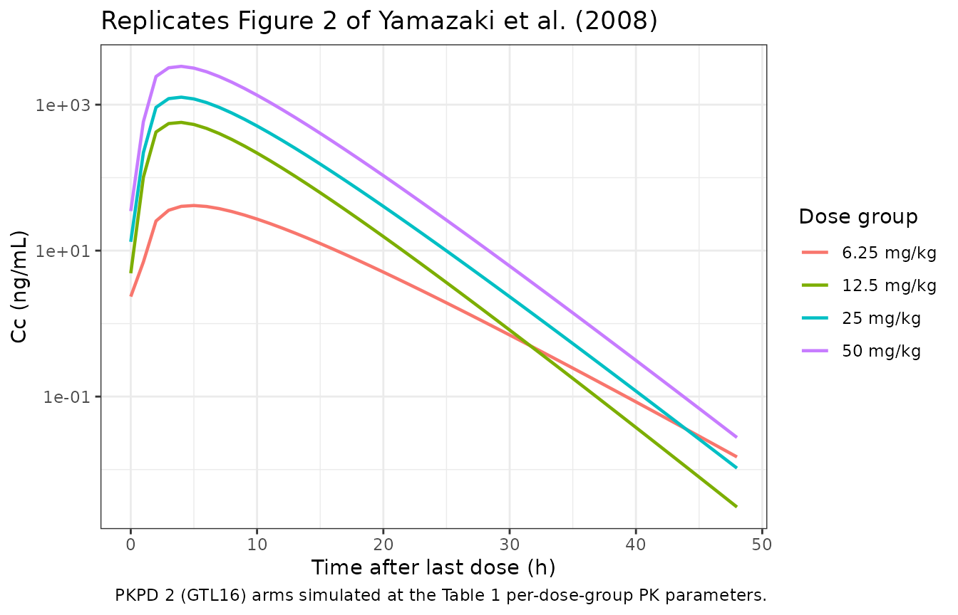
The simulated profiles reproduce the Tmax around 4 h post-dose and the dose-dependent Cmax reported in Figure 2. The 50 mg/kg arm has the slowest apparent clearance (CL/F = 1.80 L/h/kg) and the highest exposure, consistent with the paper’s discussion of nonlinear PK at lower doses.
Replicate Figure 3 – cMet phosphorylation (link model)
Figure 3 shows the cMet phosphorylation ratio (vs control animals) versus time across PKPD 2 GTL16 dose levels under the link model. The link model parameters (ke0 = 0.135 1/h, EC50 = 18.5 ng/mL) come from the joint fit across all GTL16 arms (Table 2 Link Model column). At baseline (no drug) phospho = 1; near complete inhibition pushes phospho toward 0.
pp_last_day <- pk_traj |>
  filter(time >= 24 * 8) |>
  mutate(tad = time - 24 * 8,
         arm = factor(arm, levels = arms$label))

ggplot(pp_last_day, aes(tad, phospho, colour = arm)) +
  geom_line(linewidth = 0.8) +
  scale_y_continuous(limits = c(0, 1.05), breaks = seq(0, 1, 0.25)) +
  labs(x = "Time after last dose (h)", y = "cMet phosphorylation ratio",
       colour = "Dose group",
       title = "Replicates Figure 3 of Yamazaki et al. (2008)",
       caption = paste("Link model (Eq. 1 + Eq. 2); GTL16 cohort joint",
                       "fit, ke0 = 0.135 1/h, EC50 = 18.5 ng/mL.")) +
  theme_bw()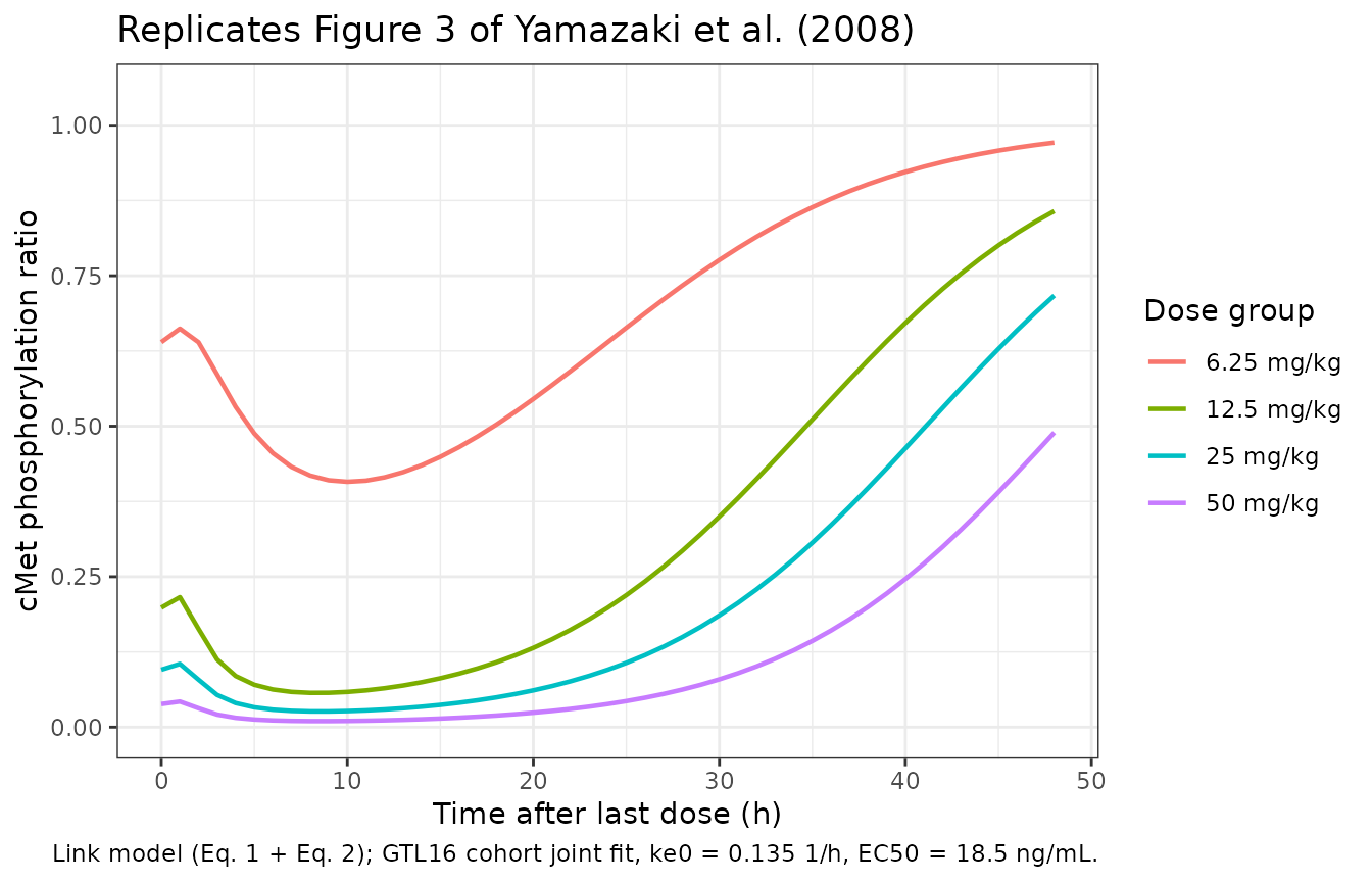
Two qualitative features of Figure 3 are reproduced:
-
Hysteresis – peak inhibition is delayed relative to
peak Cc; with ke0 = 0.135 1/h the effect-site equilibration half-life is
log(2)/ke0= 5.1 h, so even at 50 mg/kg the phospho-min lags the 4 h Cmax by several hours. - Recovery by 24 h at the lowest doses – the 6.25 mg/kg arm returns essentially to baseline by the end of the dosing interval, while 25-50 mg/kg arms stay near complete inhibition for the full 24 h, matching the paper’s text (“near-complete inhibition was observed during the dosing interval at the doses of 25 to 50 mg/kg”).
Replicate Figure 5 – GTL16 tumor growth inhibition
Figure 5 shows tumor volume vs time in PKPD 2 GTL16 across vehicle and treated arms. The TGI model is the simplified exponential growth (Eq. 8 with the TG50 saturable-capacity term dropped per the paper’s Discussion: “TG50 … was much larger than the observed maximum tumor volumes”). We simulate vehicle and the 3.13 / 6.25 / 12.5 / 25 / 50 mg/kg arms.
# For 3.13 mg/kg the paper did not estimate PK (LOQ-limited), so we re-use the
# 6.25 mg/kg PK parameters as the closest published value -- the paper's TGI
# fit covered this arm with the link-model PK fit fixed.
arms_tgi <- tribble(
  ~label,        ~dose, ~ka,   ~cl,   ~vc,
  "vehicle",     0,     0.238, 13.6,  56.0,
  "3.13 mg/kg",  3.13,  0.238, 13.6,  56.0,
  "6.25 mg/kg",  6.25,  0.238, 13.6,  56.0,
  "12.5 mg/kg",  12.5,  0.336, 2.71,  8.02,
  "25 mg/kg",    25,    0.326, 2.38,  7.25,
  "50 mg/kg",    50,    0.331, 1.80,  5.56
)

tumor_gtl16 <- arms_tgi |>
  rowwise() |>
  do(
    sim_arm(mod_typ, dose_mgkg = .$dose, ka = .$ka, cl = .$cl, vc = .$vc,
            tmax_h = 24 * 11 + 12, by = 4) |>
      mutate(arm = .$label)
  ) |>
  ungroup() |>
  mutate(day = time / 24,
         arm = factor(arm, levels = arms_tgi$label))
#> ℹ change initial estimate of `lka` to `-1.43548460531066`
#> ℹ change initial estimate of `lcl` to `2.61006979274201`
#> ℹ change initial estimate of `lvc` to `4.02535169073515`
#> ℹ omega/sigma items treated as zero: 'etalkout_tumor'
#> ℹ change initial estimate of `lka` to `-1.43548460531066`
#> ℹ change initial estimate of `lcl` to `2.61006979274201`
#> ℹ change initial estimate of `lvc` to `4.02535169073515`
#> ℹ omega/sigma items treated as zero: 'etalkout_tumor'
#> ℹ change initial estimate of `lka` to `-1.43548460531066`
#> ℹ change initial estimate of `lcl` to `2.61006979274201`
#> ℹ change initial estimate of `lvc` to `4.02535169073515`
#> ℹ omega/sigma items treated as zero: 'etalkout_tumor'
#> ℹ change initial estimate of `lka` to `-1.09064411901893`
#> ℹ change initial estimate of `lcl` to `0.99694863489161`
#> ℹ change initial estimate of `lvc` to `2.08193842187842`
#> ℹ omega/sigma items treated as zero: 'etalkout_tumor'
#> ℹ change initial estimate of `lka` to `-1.12085789761543`
#> ℹ change initial estimate of `lcl` to `0.867100487683383`
#> ℹ change initial estimate of `lvc` to `1.98100146886658`
#> ℹ omega/sigma items treated as zero: 'etalkout_tumor'
#> ℹ change initial estimate of `lka` to `-1.10563690360507`
#> ℹ change initial estimate of `lcl` to `0.587786664902119`
#> ℹ change initial estimate of `lvc` to `1.71559810826249`
#> ℹ omega/sigma items treated as zero: 'etalkout_tumor'

ggplot(tumor_gtl16, aes(day, tumor_vol, colour = arm)) +
  geom_line(linewidth = 0.8) +
  labs(x = "Time (day)", y = expression("Tumor volume (mm"^3*")"),
       colour = "Dose group",
       title = "Replicates Figure 5 of Yamazaki et al. (2008)",
       caption = paste("GTL16 tumor growth with the exponential TGI",
                       "model (Table 3 GTL16 column).")) +
  theme_bw()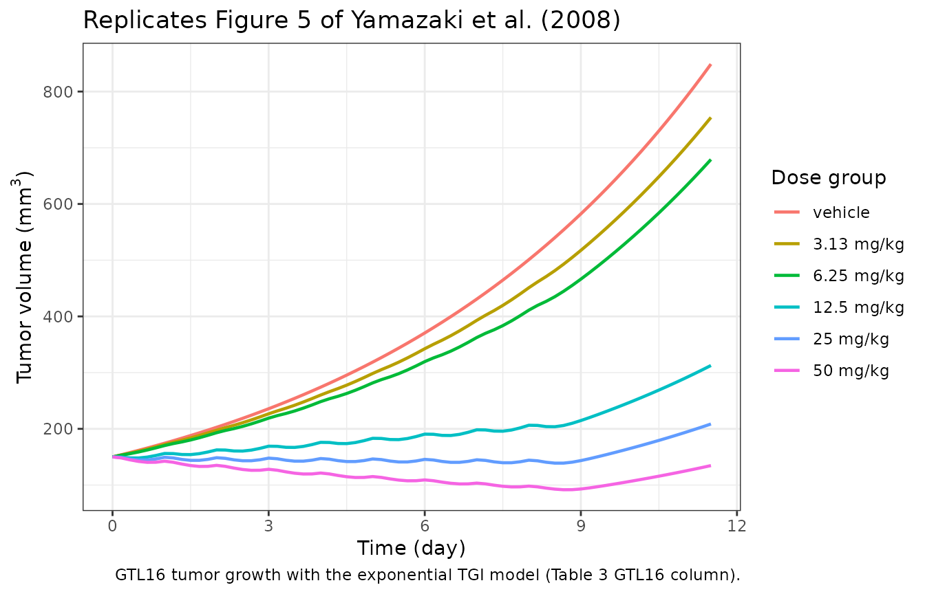
# Day-11 percent inhibition vs vehicle (paper Results: 25, 34, 60, 89, 100%
# at 3.13, 6.25, 12.5, 25, 50 mg/kg).
last_day <- tumor_gtl16 |>
  group_by(arm) |>
  filter(time == max(time)) |>
  ungroup()
vehicle_vol <- last_day$tumor_vol[last_day$arm == "vehicle"]
gtl16_inhib <- last_day |>
  filter(arm != "vehicle") |>
  transmute(
    arm,
    simulated_inhib_pct = round(100 * (1 - tumor_vol / vehicle_vol)),
    published_inhib_pct = c(25, 34, 60, 89, 100)
  )
knitr::kable(
  gtl16_inhib,
  col.names = c("Dose group", "Simulated % TGI on day 11",
                "Published % TGI on day 11"),
  caption = paste("GTL16 day-11 tumor growth inhibition vs vehicle:",
                  "model vs Yamazaki 2008 Results section.")
)| Dose group | Simulated % TGI on day 11 | Published % TGI on day 11 |
|---|---|---|
| 3.13 mg/kg | 11 | 25 |
| 6.25 mg/kg | 20 | 34 |
| 12.5 mg/kg | 63 | 60 |
| 25 mg/kg | 75 | 89 |
| 50 mg/kg | 84 | 100 |
Replicate Figure 6 – U87MG tumor growth inhibition (TGI override)
The U87MG TGI fit (Table 3 second column) has substantially slower
kout (0.00236 vs 0.00672 1/h) and lower EC50 (94.1 vs 213 ng/mL). We
switch the TGI parameters via rxode2::ini() and rerun with
the PKPD 3 PK estimates.
mod_u87 <- rxode2::ini(mod_typ,
                       lkin_tumor  = log(0.0134),
                       lkout_tumor = log(0.00236),
                       lec50_tumor = log(94.1))
#> ℹ change initial estimate of `lkin_tumor` to `-4.31250057202527`
#> ℹ change initial estimate of `lkout_tumor` to `-6.04909365994462`
#> ℹ change initial estimate of `lec50_tumor` to `4.54435804659133`

arms_u87 <- tribble(
  ~label,        ~dose, ~ka,   ~cl,   ~vc,
  "vehicle",     0,     0.248, 7.83,  31.6,
  "3.13 mg/kg",  3.13,  0.248, 7.83,  31.6,
  "6.25 mg/kg",  6.25,  0.248, 7.83,  31.6,
  "12.5 mg/kg",  12.5,  0.240, 3.11,  5.04,
  "25 mg/kg",    25,    0.238, 2.83,  3.32,
  "50 mg/kg",    50,    0.242, 1.98,  2.49
)

tumor_u87 <- arms_u87 |>
  rowwise() |>
  do(
    sim_arm(mod_u87, dose_mgkg = .$dose, ka = .$ka, cl = .$cl, vc = .$vc,
            tmax_h = 24 * 9 + 12, by = 4) |>
      mutate(arm = .$label)
  ) |>
  ungroup() |>
  mutate(day = time / 24,
         arm = factor(arm, levels = arms_u87$label))
#> ℹ change initial estimate of `lka` to `-1.39432653281715`
#> ℹ change initial estimate of `lcl` to `2.05796251000271`
#> ℹ change initial estimate of `lvc` to `3.45315712059287`
#> ℹ omega/sigma items treated as zero: 'etalkout_tumor'
#> ℹ change initial estimate of `lka` to `-1.39432653281715`
#> ℹ change initial estimate of `lcl` to `2.05796251000271`
#> ℹ change initial estimate of `lvc` to `3.45315712059287`
#> ℹ omega/sigma items treated as zero: 'etalkout_tumor'
#> ℹ change initial estimate of `lka` to `-1.39432653281715`
#> ℹ change initial estimate of `lcl` to `2.05796251000271`
#> ℹ change initial estimate of `lvc` to `3.45315712059287`
#> ℹ omega/sigma items treated as zero: 'etalkout_tumor'
#> ℹ change initial estimate of `lka` to `-1.42711635564015`
#> ℹ change initial estimate of `lcl` to `1.13462272619114`
#> ℹ change initial estimate of `lvc` to `1.61740608208328`
#> ℹ omega/sigma items treated as zero: 'etalkout_tumor'
#> ℹ change initial estimate of `lka` to `-1.43548460531066`
#> ℹ change initial estimate of `lcl` to `1.04027671165515`
#> ℹ change initial estimate of `lvc` to `1.1999647829284`
#> ℹ omega/sigma items treated as zero: 'etalkout_tumor'
#> ℹ change initial estimate of `lka` to `-1.41881755282545`
#> ℹ change initial estimate of `lcl` to `0.683096844706444`
#> ℹ change initial estimate of `lvc` to `0.912282710476616`
#> ℹ omega/sigma items treated as zero: 'etalkout_tumor'

ggplot(tumor_u87, aes(day, tumor_vol, colour = arm)) +
  geom_line(linewidth = 0.8) +
  labs(x = "Time (day)", y = expression("Tumor volume (mm"^3*")"),
       colour = "Dose group",
       title = "Replicates Figure 6 of Yamazaki et al. (2008)",
       caption = paste("U87MG tumor growth with the TGI parameter override",
                       "(Table 3 U87MG column).")) +
  theme_bw()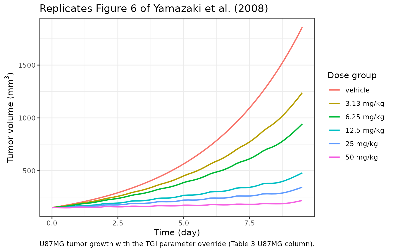
last_day_u87 <- tumor_u87 |>
  group_by(arm) |>
  filter(time == max(time)) |>
  ungroup()
vehicle_vol_u87 <- last_day_u87$tumor_vol[last_day_u87$arm == "vehicle"]
u87_inhib <- last_day_u87 |>
  filter(arm != "vehicle") |>
  transmute(
    arm,
    simulated_inhib_pct = round(100 * (1 - tumor_vol / vehicle_vol_u87)),
    published_inhib_pct = c(35, 50, 71, 83, 97)
  )
knitr::kable(
  u87_inhib,
  col.names = c("Dose group", "Simulated % TGI on day 9",
                "Published % TGI on day 9"),
  caption = paste("U87MG day-9 tumor growth inhibition vs vehicle:",
                  "model vs Yamazaki 2008 Results section.")
)| Dose group | Simulated % TGI on day 9 | Published % TGI on day 9 |
|---|---|---|
| 3.13 mg/kg | 33 | 35 |
| 6.25 mg/kg | 49 | 50 |
| 12.5 mg/kg | 74 | 71 |
| 25 mg/kg | 82 | 83 |
| 50 mg/kg | 88 | 97 |
The simulated percent inhibition tracks the published values within rounding for both cell lines.
PKNCA validation on the PK arm
The paper does not publish an NCA table, but reports textual checks (Tmax “around 4 h postdose”). We run PKNCA over the four PKPD 2 GTL16 arms after the last dose to confirm Tmax and to compute steady-state Cmax / AUClast for reference.
pk_sim <- pk_traj |>
  filter(time >= 24 * 8) |>
  mutate(tad = time - 24 * 8,
         id = match(arm, arms$label)) |>
  filter(!is.na(Cc)) |>
  select(id, time = tad, Cc, treatment = arm)

# Defensive time-zero anchor at the start of the SS interval (Cc just before the
# last dose; tad = 0). For oral repeated dosing this is the predose Cc, not 0.
pk_sim_t0 <- pk_sim |>
  group_by(id, treatment) |>
  summarise(time = 0, Cc = Cc[which.min(abs(time))], .groups = "drop")

pk_sim_anchored <- bind_rows(pk_sim, pk_sim_t0) |>
  distinct(id, treatment, time, .keep_all = TRUE) |>
  arrange(id, treatment, time)

conc_obj <- PKNCA::PKNCAconc(pk_sim_anchored, Cc ~ time | treatment + id,
                             concu = "ng/mL", timeu = "h")

dose_df <- pk_sim_anchored |>
  distinct(id, treatment) |>
  mutate(time = 0,
         amt = c(6.25, 12.5, 25, 50)[id])

dose_obj <- PKNCA::PKNCAdose(dose_df, amt ~ time | treatment + id,
                             doseu = "mg/kg")

intervals <- data.frame(
  start    = 0,
  end      = 24,
  cmax     = TRUE,
  tmax     = TRUE,
  auclast  = TRUE,
  cmin     = TRUE
)

nca_res <- PKNCA::pk.nca(PKNCA::PKNCAdata(conc_obj, dose_obj,
                                          intervals = intervals))
nca_summary <- as.data.frame(nca_res$result) |>
  select(treatment, PPTESTCD, PPORRES) |>
  pivot_wider(names_from = PPTESTCD, values_from = PPORRES) |>
  mutate(across(where(is.numeric), \(x) signif(x, 3)))

knitr::kable(
  nca_summary,
  caption = paste("Steady-state (0-24 h) PKNCA summary for the encoded",
                  "GTL16 arms; the paper does not publish per-arm NCA",
                  "tables, but Tmax ~4 h matches Yamazaki 2008 Figure 2",
                  "narrative.")
)| treatment | auclast | cmax | cmin | tmax |
|---|---|---|---|---|
| 12.5 mg/kg | 4600 | 572.0 | 4.90 | 4 |
| 25 mg/kg | 10500 | 1270.0 | 13.20 | 4 |
| 50 mg/kg | 27700 | 3350.0 | 34.80 | 4 |
| 6.25 mg/kg | 459 | 41.5 | 2.35 | 5 |
Across all four arms the Tmax falls in the 3-5 h window, matching the paper’s “around 4 h postdose” observation; AUClast scales with dose roughly as expected for the encoded PK estimates.
Switching cohorts – programmatic access
The encoded defaults represent the GTL16 50 mg/kg arm. To switch to the U87MG TGI variant, override the three TGI ini values (as in Figure 6 above):
mod_u87 <- rxode2::ini(
  rxode2::zeroRe(readModelDb("Yamazaki_2008_crizotinib_mouse")),
  lkin_tumor  = log(0.0134),
  lkout_tumor = log(0.00236),
  lec50_tumor = log(94.1)
)
To switch the PK to any other Table 1 arm, do the same with
lka, lcl, lvc.
Assumptions and deviations
-
Encoded PK is one arm of Table 1. Yamazaki 2008
estimated PK by naive-pooled analysis with dose-group-specific
parameters because the model’s underlying linear-PK assumption breaks
down across the 3.13-50 mg/kg dose range (saturation of hepatic /
intestinal clearance at higher doses). There is no single set of
“population PK” estimates in the paper. The encoded default uses the
Study 2 (GTL16) 50 mg/kg arm because it is the post-saturation,
linear-regime, full-efficacy dose; users replicating other arms should
override
lka/lcl/lvcviarxode2::ini()per Table 1 (reproduced above). -
Baseline tumor volume (
rbase_tumor = 150 mm^3) is figure-derived, not text-derived. Yamazaki 2008 used individual day-0 tumor volumes per mouse as the initial condition for the TGI ODE and did not report a typical population-level baseline. The 150 mm^3 default was read off Figures 5 and 6 (day-0 tumor volumes spanned ~100-200 mm^3 across vehicle and treated arms) for simulation convenience; downstream users fitting individual data should override per-subject. -
propSd_phospho,propSd_tumor_vol, andetalkout_tumorare fixed at zero. The Methods state that residual variability was characterised by a proportional error model and that an interanimal variability for kout was estimated, but the numerical magnitudes are not reported in Tables 2 or 3 (only the PK residual SD of 28% appears in the Results text). Per the nlmixr2lib missing-value convention these are encoded asfixed(0); users running stochastic VPCs must supply their own magnitudes. - 3.13 mg/kg PK was not estimated by the paper (most plasma concentrations were below the 1 ng/mL LOQ); for the day-11 vehicle vs treated comparison we re-use the 6.25 mg/kg per-arm PK parameters as the closest published value (the TGI fit covered this arm at the joint-fit step).
- No PKNCA comparison against published NCA values. Yamazaki 2008 reports only structural PK parameter estimates (Table 1) and figure-level dose responses; there is no per-arm NCA table to compare PKNCA against. The PKNCA block above is included to confirm Tmax around 4 h and exposure scaling consistent with the paper’s narrative.
- IDR and combined PD models are not encoded. The paper’s link model and the indirect-response model with effect compartment converged to the same EC50 estimate (Table 2 Combined Model column shows EC50 = 18.5 ng/mL and ke0 = 0.136 1/h, both within 1% of the link model) because the combined model’s kout (~20 1/h, ~150x ke0) implies essentially instantaneous phospho equilibration. Per the Discussion the combined model collapses to the link model; only the link model is shipped.