Voriconazole (Kim 2019)
Source:vignettes/articles/Kim_2019_voriconazole.Rmd
Kim_2019_voriconazole.RmdModel and source
#> ℹ parameter labels from comments will be replaced by 'label()'Citation: Kim Y, Rhee SJ, Park WB, Yu KS, Jang IJ, Lee S. A personalized CYP2C19 phenotype-guided dosing regimen of voriconazole using a population pharmacokinetic analysis. J Clin Med. 2019 Feb 10;8(2):227. doi:10.3390/jcm8020227. PMCID PMC6406770.
Description: Three-compartment population pharmacokinetic model for intravenous and oral voriconazole in Korean healthy volunteers and patients (Kim 2019), with first-order absorption, an absorption lag time, a logit-scale absolute bioavailability, and a mechanistic auto-inhibition compartment that makes clearance time-dependent: CL(t) = CL0 * [RCLF + (1 - RCLF) * IC50 / (IC50 + Cinh)], so clearance decays from CL0 toward the non-inhibitable floor CL0 * RCLF as drug accumulates in the inhibition compartment. CYP2C19 metabolizer phenotype acts on both CL0 and RCLF, body weight on CL0, the first peripheral volume and the first inter-compartmental clearance, and a CTCAE grade >= 3 liver function abnormality on CL0.
Article: https://doi.org/10.3390/jcm8020227 (open access; PMCID PMC6406770)
Supplement (Tables S1-S3, Figures S1-S2): https://www.mdpi.com/2077-0383/8/2/227/s1
Voriconazole has famously non-linear, highly variable
pharmacokinetics. Kim 2019 is the first population model to attribute
that non-linearity to a mechanistic auto-inhibition rather than
to Michaelis-Menten elimination: an empirical inhibition compartment
accumulates a concentration Cinh that progressively shuts
down the drug’s own clearance, and the CYP2C19 metabolizer phenotype
modulates both the starting clearance and the floor it decays to.
Population
The model was built on 1,828 plasma voriconazole concentrations from 193 Korean subjects pooled across five studies run at Seoul National University Hospital (Kim 2019 Table 1 and Table S1): 93 healthy volunteers contributing 1,579 intensively sampled observations (studies 1-4) and 100 patients contributing 249 sparse therapeutic-drug-monitoring observations (study 5). Median age was 34 years (range 18-80; 26 in the healthy volunteers, 59 in the patients) and median body weight 66.0 kg (range 40.8-88.5; 70.3 kg healthy, 59.4 kg patients). 164 subjects (85%) were male. The CYP2C19 phenotype split was 75 extensive metabolizers (39%), 70 intermediate metabolizers (36%) and 48 poor metabolizers (25%). CTCAE v4.0 liver function abnormality was grade 0 in 165 subjects (85.5%) and grade >= 3 in only 6. Doses ranged from single 200 mg intravenous and 200-400 mg oral doses in the volunteer studies to a 6 mg/kg IV or 400 mg oral twice-daily loading day followed by TDM-guided maintenance in the patients.
The same information is available programmatically via
readModelDb("Kim_2019_voriconazole")()$population.
Source trace
Each ini() entry in
inst/modeldb/specificDrugs/Kim_2019_voriconazole.R carries
an in-file comment pointing at its source location; they are collected
here for review.
| Equation / parameter | Value | Source location |
|---|---|---|
lka |
1.23 1/h | Table 2, Ka (RSE 15.4%) |
ltlag |
0.237 h | Table 2, ALAG1 (RSE 1.8%) |
logitfdepot |
logit(0.876) = 1.955 | Table 2, F1 = 0.876 (RSE 2.3%); Methods states F was
estimated with a logit model |
lvc |
35.7 L | Table 2, V2 (RSE 15.7%) |
lcl |
45.3 L/h | Table 2, CL (RSE 5.8%) |
lvp |
58.9 L | Table 2, V3 (RSE 6.2%) |
lq |
10.9 L/h | Table 2, Q2 (RSE 8.0%) |
lvp2 |
25.4 L | Table 2, V4 (RSE 16.7%) |
lq2 |
54.6 L/h | Table 2, Q3 (RSE 45.4%) |
lfcl_noinh |
0.162 | Table 2, RCLF (RSE 9.7%) |
lic50 |
0.01 mg/L, fixed | Table 2, IC50 = “0.01 FIX” |
lke0 |
0.002 1/h | Table 2, KIC (RSE 14.9%) |
e_wt_cl |
0.595 | Table 3, body weight exponent for CL (RSE 31.8%) |
e_wt_vp |
2.2 | Table 3, body weight exponent for V3 (RSE 20.0%) |
e_wt_q |
2.56 | Table 3, body weight exponent for Q2 (RSE 18.1%) |
e_cyp2c19_im_cl |
-0.186 | Table 3, “Effect on CL”, intermediate metabolizer (RSE 29.5%) |
e_cyp2c19_pm_cl |
-0.746 | Table 3, “Effect on CL”, poor metabolizer (RSE 10.9%) |
e_hepimp_sev_cl |
-0.75 | Table 3, “Effect on CL”, liver function grade >= 3 (RSE 49.3%) |
e_cyp2c19_im_fcl_noinh |
-0.51 | Table 3, “Effect on RCLF”, intermediate metabolizer (RSE 27.5%) |
e_cyp2c19_pm_fcl_noinh |
-0.44 | Table 3, “Effect on RCLF”, poor metabolizer (RSE 42.3%) |
| IIV (V2, CL, V3, Q2, Ka, F1, RCLF) | 40.2 / 21.4 / 20.6 / 28.8 / 87.8 / 84.4 / 54.4 %CV | Table 2, “Inter-individual variability”; converted with
omega^2 = log(CV^2 + 1)
|
| OMEGA off-diagonals | 0.0116 / -0.0117 / -0.0734 / -0.0119 / 0.008 / 0.0345 | Table 2, “Correlation between …” rows; footnote b identifies them as covariance estimates |
addSdHealthy / addSdPatient
|
0.208 / 0.799 mg/L | Table 2, “Residual variability” (RSE 8.4% / 6.7%) |
CL = CL0 * INH |
n/a | Equation 1 |
INH = RCLF + (1 - RCLF) * (1 - Cinh/(IC50 + Cinh)) |
n/a | Equation 2, and the Figure 1 caption |
d/dt(effect) = KIC * Cc |
n/a | Figure 1 (a single KIC arrow into the inhibition
compartment, no return or elimination arrow) and Table 2
(KIC, “rate constant into inhibition compartment”; no
second rate constant reported) |
| Reference weight 70 kg | n/a | Methods, “Population pharmacokinetic analysis”: covariates normalized to “a generally accepted typical value (e.g., 70 kg for body weight)” |
Structural checks against the published typical values
These are deterministic consequences of the ini() block,
so they are asserted exactly (to the precision the paper prints).
mod <- nlmixr2lib::readModelDb("Kim_2019_voriconazole")
mod_typ <- mod |> rxode2::zeroRe()
#> ℹ parameter labels from comments will be replaced by 'label()'
#> Warning: No sigma parameters in the model

pheno_cov <- function(ph, wt = 70, hep = 0, healthy = 1) {
  data.frame(
    WT = wt,
    CYP2C19_IM = as.numeric(ph == "IM"),
    CYP2C19_PM = as.numeric(ph == "PM"),
    HEPIMP_SEV = hep,
    DIS_HEALTHY = healthy
  )
}

probe_ev <- rxode2::et(amt = 400, cmt = "depot", time = 0) |>
  rxode2::et(amt = 400, cmt = "depot", time = 12) |>
  rxode2::et(amt = 200, cmt = "depot", time = seq(24, 156, by = 12)) |>
  rxode2::et(seq(0, 168, by = 0.5), cmt = "central")

solve_typ <- function(ph, wt = 70, hep = 0) {
  rxode2::rxSolve(
    mod_typ, probe_ev, pheno_cov(ph, wt = wt, hep = hep),
    returnType = "data.frame", useLinCmt = FALSE
  )
}

typ <- lapply(c(EM = "EM", IM = "IM", PM = "PM"), solve_typ)
#> ℹ omega/sigma items treated as zero: 'etalvc', 'etalcl', 'etalvp', 'etalq', 'etalka', 'etalogitfdepot', 'etalfcl_noinh'
#> ℹ omega/sigma items treated as zero: 'etalvc', 'etalcl', 'etalvp', 'etalq', 'etalka', 'etalogitfdepot', 'etalfcl_noinh'
#> ℹ omega/sigma items treated as zero: 'etalvc', 'etalcl', 'etalvp', 'etalq', 'etalka', 'etalogitfdepot', 'etalfcl_noinh'

structural <- tibble::tibble(
  phenotype = names(typ),
  cl0 = vapply(typ, function(s) s$cl0[1], numeric(1)),
  rclf = vapply(typ, function(s) s$fcl_noinh[1], numeric(1)),
  inh_t0 = vapply(typ, function(s) s$inh[1], numeric(1)),
  cl_floor = cl0 * rclf,
  published_cl0 = c(45.3, 37.6, 21.5)
)

structural |>
  dplyr::rename(
    "CYP2C19 phenotype" = phenotype,
    "CL0 (L/h)" = cl0,
    "RCLF" = rclf,
    "INH at t = 0" = inh_t0,
    "CL0 x RCLF (L/h)" = cl_floor,
    "Published CL0 (L/h)" = published_cl0
  ) |>
  knitr::kable(
    digits = c(0, 2, 4, 6, 2, 1),
    caption = paste(
      "Typical-value clearance parameters by CYP2C19 phenotype at the 70 kg",
      "reference weight. Published CL0 values are Kim 2019 Results 3.2."
    )
)| CYP2C19 phenotype | CL0 (L/h) | RCLF | INH at t = 0 | CL0 x RCLF (L/h) | Published CL0 (L/h) |
|---|---|---|---|---|---|
| EM | 45.30 | 0.1620 | 1 | 7.34 | 45.3 |
| IM | 37.61 | 0.0973 | 1 | 3.66 | 37.6 |
| PM | 21.48 | 0.1043 | 1 | 2.24 | 21.5 |
# CL0 by phenotype reproduces Kim 2019 Results 3.2 (45.3 / 37.6 / 21.5 L/h) to
# the printed precision. Deterministic -- assert tightly.
stopifnot(max(abs(structural$cl0 - structural$published_cl0)) < 0.05)

# RCLF by phenotype. Kim 2019 Results 3.2 prints the EM value as 0.162 and the
# IM/PM pair as the range "0.097-0.104".
stopifnot(
  abs(structural$rclf[structural$phenotype == "EM"] - 0.162) < 5e-4,
  abs(min(structural$rclf[structural$phenotype != "EM"]) - 0.097) < 5e-4,
  abs(max(structural$rclf[structural$phenotype != "EM"]) - 0.104) < 5e-4
)

# INH must be exactly 1 before any drug has entered the inhibition compartment,
# so the model starts at the uninhibited clearance. Machine-precision identity.
stopifnot(max(abs(structural$inh_t0 - 1)) < 1e-12)

# The CTCAE grade >= 3 liver-function coefficient multiplies CL0 by exp(-0.75).
hep_cl0 <- solve_typ("EM", hep = 1)$cl0[1]
#> ℹ omega/sigma items treated as zero: 'etalvc', 'etalcl', 'etalvp', 'etalq', 'etalka', 'etalogitfdepot', 'etalfcl_noinh'
stopifnot(abs(hep_cl0 / structural$cl0[structural$phenotype == "EM"] - exp(-0.75)) < 1e-10)

# The clearance must genuinely be time-varying, i.e. the solve used the ODE
# system rather than an auto-converted linear-compartment solution. Without
# this, every check below could pass against a constant-CL model.
stopifnot(
  vapply(typ, function(s) diff(range(s$cl)) / s$cl[1], numeric(1)) > 0.5,
  is.null(rxode2::rxode(mod)$linCmt)
)
#> ℹ parameter labels from comments will be replaced by 'label()'
Clearance falls to 16.2% of its starting value in extensive metabolizers, which is exactly the paper’s headline “time-dependent inhibition of clearance to 16.2% of its original value”.
Mass balance
Appending an accumulator state for eliminated drug turns the mass balance into an exact identity rather than a trapezoidal approximation: everything that was absorbed must be either eliminated or still resident in one of the three disposition compartments.
mod_mb <- mod_typ |> rxode2::model(d / dt(a_eliminated) <- cl * Cc, append = TRUE)

mb <- rxode2::rxSolve(
  mod_mb, probe_ev, pheno_cov("EM"),
  returnType = "data.frame", useLinCmt = FALSE
)
#> ℹ omega/sigma items treated as zero: 'etalvc', 'etalcl', 'etalvp', 'etalq', 'etalka', 'etalogitfdepot', 'etalfcl_noinh'
mb_end <- mb[nrow(mb), ]

dose_total <- sum(c(400, 400, rep(200, 12)))
absorbed <- dose_total * 0.876
accounted <- with(
  mb_end,
  a_eliminated + central + peripheral1 + peripheral2 + depot
)

cat(sprintf(
  "F * dose = %.6f mg; eliminated + resident = %.6f mg; relative error = %.2e\n",
  absorbed, accounted, abs(accounted / absorbed - 1)
))
#> F * dose = 2803.200000 mg; eliminated + resident = 2803.200165 mg; relative error = 5.89e-08
stopifnot(abs(accounted / absorbed - 1) < 1e-6)
Replicating Supplementary Figure S1, and the Table 3 / Discussion conflict
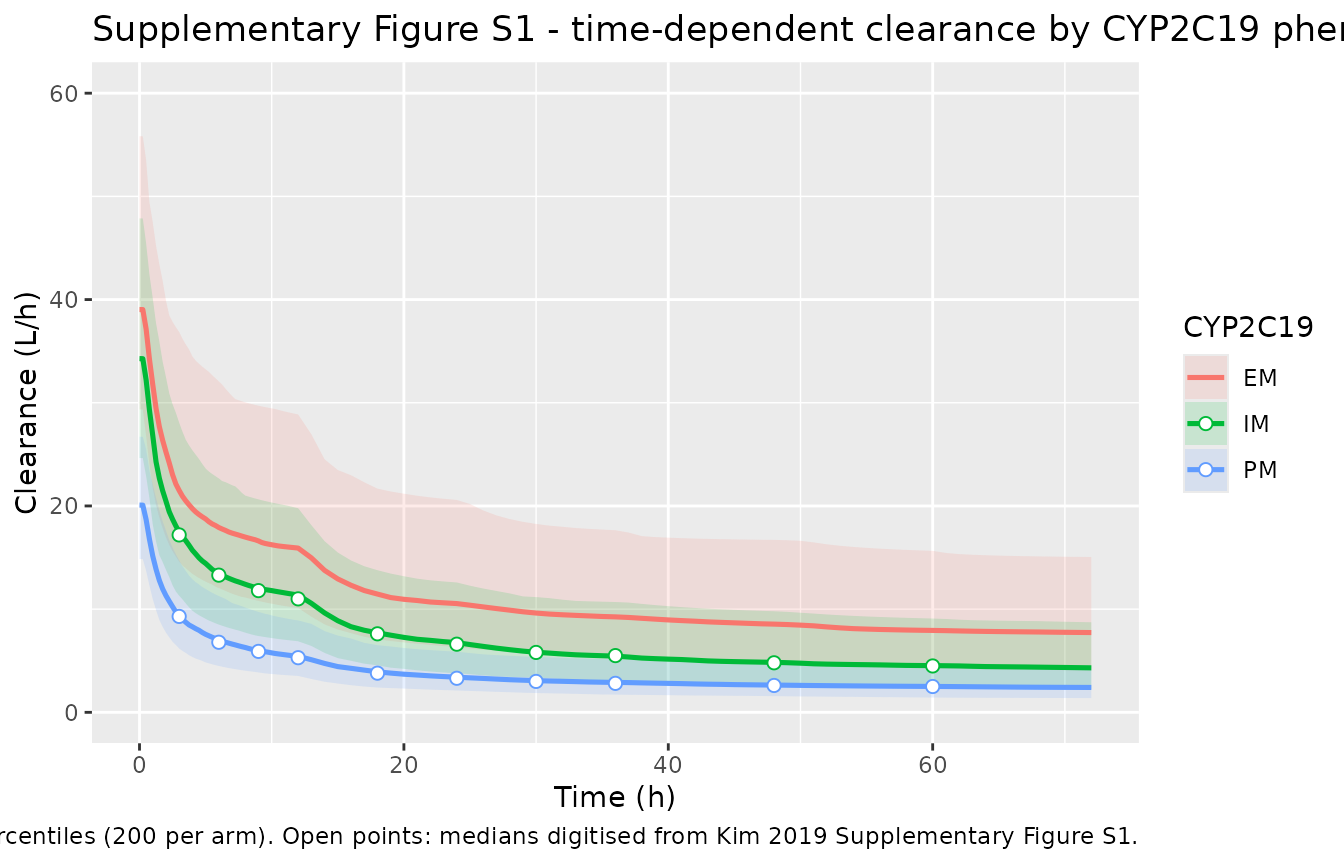
Supplementary Figure S1 plots predicted voriconazole clearance against time for the three CYP2C19 phenotypes under the standard oral regimen. Its three median curves were digitised from the published figure (axis calibration from the tick marks; the median line is the solid curve, distinguished from the hatched 10th-90th percentile band by its line width).
This figure is doing real work here, because Kim 2019
contradicts itself about which CYP2C19 coefficient belongs to which
phenotype on RCLF. Table 3 gives the RCLF effects as IM = -0.51
and PM = -0.44, i.e. RCLF_IM = 0.162 * exp(-0.51) = 0.0973
and RCLF_PM = 0.162 * exp(-0.44) = 0.1043. But the
Discussion states that clearance “changes from 45.3 to 7.3 L/h in
CYP2C19 EMs, from 37.6 to 3.9 L/h in IMs, and from 21.5 to 2.1 L/h in
PMs” – and while the EM pair is exactly
CL0 * RCLF = 45.3 * 0.162 = 7.34, the IM and PM figures are
only reproduced by pairing each phenotype’s CL0 with the other
phenotype’s RCLF (37.61 * 0.1043 = 3.92,
21.48 * 0.0973 = 2.09). Table 3 as printed gives 3.66 and
2.24 instead.
Figure S1 settles it. The mechanism is directional and unambiguous:
poor metabolizers have the higher exposure, therefore the larger
Cinh, therefore an inhibition factor closer to its floor
than intermediate metabolizers at the same time point. That constrains
the ratio CL_IM(t) / CL_PM(t), which – being a ratio
between two phenotypes sharing the same covariate distribution – is
independent of body weight and of any common scaling error in the
digitisation.
# Median CL-versus-time curves digitised from Kim 2019 Supplementary Figure S1
# (600 dpi render; y axis 0-60 L/h over 7 ticks, x axis 0-72 h over 7 ticks).
fig_s1 <- tibble::tribble(
  ~time, ~IM, ~PM,
  3, 17.191, 9.294,
  6, 13.294, 6.791,
  9, 11.796, 5.906,
  12, 10.996, 5.294,
  18, 7.609, 3.796,
  24, 6.604, 3.302,
  30, 5.804, 2.996,
  36, 5.498, 2.809,
  48, 4.800, 2.604,
  60, 4.494, 2.502
)
# Typical-value (zeroRe) clearance trajectories, so this comparison carries no
# cohort sampling noise at all and can be gated tightly.
cl_at <- function(sol, times) approx(sol$time, sol$cl, times)$y

# Variant B: the assignment implied by the Discussion sentence, i.e. the two
# RCLF coefficients swapped relative to Table 3.
mod_swapped <- mod_typ |>
  rxode2::ini(e_cyp2c19_im_fcl_noinh = -0.44, e_cyp2c19_pm_fcl_noinh = -0.51)
#> ℹ change initial estimate of `e_cyp2c19_im_fcl_noinh` to `-0.44`
#> ℹ change initial estimate of `e_cyp2c19_pm_fcl_noinh` to `-0.51`

solve_swapped <- function(ph) {
  rxode2::rxSolve(
    mod_swapped, probe_ev, pheno_cov(ph),
    returnType = "data.frame", useLinCmt = FALSE
  )
}

ratio_obs <- fig_s1$IM / fig_s1$PM
ratio_table <- cl_at(typ$IM, fig_s1$time) / cl_at(typ$PM, fig_s1$time)
ratio_swap <- cl_at(solve_swapped("IM"), fig_s1$time) /
  cl_at(solve_swapped("PM"), fig_s1$time)
#> ℹ omega/sigma items treated as zero: 'etalvc', 'etalcl', 'etalvp', 'etalq', 'etalka', 'etalogitfdepot', 'etalfcl_noinh'
#> ℹ omega/sigma items treated as zero: 'etalvc', 'etalcl', 'etalvp', 'etalq', 'etalka', 'etalogitfdepot', 'etalfcl_noinh'

arb <- tibble::tibble(
  time = fig_s1$time,
  figure = ratio_obs,
  table3 = ratio_table,
  swapped = ratio_swap,
  dev_table3 = 100 * (ratio_table / ratio_obs - 1),
  dev_swapped = 100 * (ratio_swap / ratio_obs - 1)
)

arb |>
  dplyr::rename(
    "Time (h)" = time,
    "Figure S1 CL(IM)/CL(PM)" = figure,
    "Table 3 as printed" = table3,
    "Discussion (swapped)" = swapped,
    "Table 3 dev (%)" = dev_table3,
    "Swapped dev (%)" = dev_swapped
  ) |>
  knitr::kable(
    digits = c(0, 3, 3, 3, 1, 1),
    caption = paste(
      "Ratio of intermediate- to poor-metabolizer clearance over time.",
      "The ratio cancels body weight and any common digitisation scale error,",
      "so it isolates which RCLF assignment the published figure supports."
    )
)| Time (h) | Figure S1 CL(IM)/CL(PM) | Table 3 as printed | Discussion (swapped) | Table 3 dev (%) | Swapped dev (%) |
|---|---|---|---|---|---|
| 3 | 1.850 | 1.897 | 1.932 | 2.5 | 4.4 |
| 6 | 1.958 | 2.008 | 2.070 | 2.6 | 5.7 |
| 9 | 1.997 | 2.083 | 2.162 | 4.3 | 8.2 |
| 12 | 2.077 | 2.139 | 2.231 | 3.0 | 7.4 |
| 18 | 2.004 | 2.002 | 2.140 | -0.1 | 6.8 |
| 24 | 2.000 | 2.001 | 2.165 | 0.1 | 8.3 |
| 30 | 1.937 | 1.949 | 2.132 | 0.6 | 10.1 |
| 36 | 1.957 | 1.937 | 2.134 | -1.0 | 9.0 |
| 48 | 1.843 | 1.883 | 2.098 | 2.1 | 13.8 |
| 60 | 1.796 | 1.840 | 2.066 | 2.4 | 15.0 |
rms <- function(x) sqrt(mean(x^2))
cat(sprintf(
  "RMS deviation of CL(IM)/CL(PM) from Figure S1: Table 3 as printed = %.1f%%, swapped = %.1f%%\n",
  rms(arb$dev_table3), rms(arb$dev_swapped)
))
#> RMS deviation of CL(IM)/CL(PM) from Figure S1: Table 3 as printed = 2.3%, swapped = 9.4%
# Deterministic (zeroRe) quantities at a fixed reference weight, so these
# bounds carry no cohort sampling noise and are reproducible across machines.
# Observed: Table 3 as printed 2.3% RMS, swapped 9.4% RMS. The bounds sit
# outside both values; do not tighten them onto the observed numbers.
stopifnot(
  rms(arb$dev_table3) < 6,
  rms(arb$dev_swapped) > 6,
  # The swapped assignment must be clearly worse, not merely different.
  rms(arb$dev_swapped) > 2 * rms(arb$dev_table3)
)
The Table 3 assignment tracks the published figure; the Discussion’s implied assignment does not. The packaged model therefore uses Table 3 as printed and records the Discussion sentence as an erratum-class transposition.
Virtual cohort
Original subject-level data are not public. Figure S1 and Figure 3 of Kim 2019 are simulations of “10,000 simulated patients”, so the cohort below is drawn to match the patient demographics of Table 1 (median weight 59.4 kg, range 40.8-86.4 kg) rather than the pooled cohort. Cohort size is 200 per CYP2C19 phenotype, the per-arm cap for validation vignettes.
# set.seed() seeds R's RNG for the covariate draw. It does NOT seed rxode2's
# simulation RNG, whose streams are partitioned per solver thread -- so every
# assertion on a cohort-derived quantity below is written as an absolute bound
# that holds for any cohort this model can produce.
set.seed(20190210)
rxode2::rxSetSeed(20190210)

n_per_arm <- 200L
phenos <- c("EM", "IM", "PM")

draw_weight <- function(n) {
  # Log-normal centred on the patients' median weight (59.4 kg), with the
  # spread truncated to the published patient range (40.8-86.4 kg).
  w <- stats::rlnorm(n, meanlog = log(59.4), sdlog = 0.20)
  pmin(pmax(w, 40.8), 86.4)
}

make_cohort <- function(pheno, n, id_offset = 0L) {
  subj <- tibble::tibble(
    id = id_offset + seq_len(n),
    phenotype = pheno,
    WT = draw_weight(n),
    CYP2C19_IM = as.numeric(pheno == "IM"),
    CYP2C19_PM = as.numeric(pheno == "PM"),
    HEPIMP_SEV = 0,
    # The published simulations are of patients, so the patient residual-error
    # magnitude applies.
    DIS_HEALTHY = 0
  )
  # Standard oral regimen: 400 mg bid for two doses, then 200 mg bid to day 7.
  doses <- subj |>
    tidyr::crossing(time = seq(0, 168, by = 12)) |>
    dplyr::mutate(
      amt = dplyr::if_else(time <= 12, 400, 200),
      evid = 1L,
      cmt = "depot"
    )
  obs <- subj |>
    tidyr::crossing(time = sort(unique(c(seq(0, 168, by = 1), seq(0, 12, by = 0.25))))) |>
    dplyr::mutate(amt = NA_real_, evid = 0L, cmt = "central")
  dplyr::bind_rows(doses, obs) |>
    dplyr::arrange(id, time, dplyr::desc(evid))
}

events <- dplyr::bind_rows(
  make_cohort("EM", n_per_arm, id_offset = 0L),
  make_cohort("IM", n_per_arm, id_offset = n_per_arm),
  make_cohort("PM", n_per_arm, id_offset = 2L * n_per_arm)
)
stopifnot(!anyDuplicated(unique(events[, c("id", "time", "evid")])))
stopifnot(dplyr::n_distinct(events$id) == 3L * n_per_arm)Replicate published figures
Supplementary Figure S1 – clearance versus time by phenotype
# Replicates Supplementary Figure S1 of Kim 2019: median (10th-90th percentile)
# predicted clearance over the first 72 h of the standard oral regimen.
cl_summary <- sim |>
  dplyr::filter(time <= 72) |>
  dplyr::group_by(phenotype, time) |>
  dplyr::summarise(
    Q10 = quantile(cl, 0.10),
    Q50 = median(cl),
    Q90 = quantile(cl, 0.90),
    .groups = "drop"
  )

ggplot(cl_summary, aes(time, Q50, colour = phenotype, fill = phenotype)) +
  geom_ribbon(aes(ymin = Q10, ymax = Q90), alpha = 0.15, colour = NA) +
  geom_line(linewidth = 0.9) +
  geom_point(
    data = fig_s1 |> tidyr::pivot_longer(c(IM, PM), names_to = "phenotype", values_to = "Q50"),
    shape = 21, size = 2, fill = "white"
  ) +
  coord_cartesian(ylim = c(0, 60)) +
  labs(
    x = "Time (h)", y = "Clearance (L/h)",
    colour = "CYP2C19", fill = "CYP2C19",
    title = "Supplementary Figure S1 - time-dependent clearance by CYP2C19 phenotype",
    caption = paste(
      "Lines/ribbons: simulated median and 10th-90th percentiles (200 per arm).",
      "Open points: medians digitised from Kim 2019 Supplementary Figure S1."
    )
  )
cl_med <- cl_summary |>
  dplyr::filter(phenotype %in% c("IM", "PM"), time %in% fig_s1$time) |>
  dplyr::select(phenotype, time, Q50) |>
  tidyr::pivot_wider(names_from = phenotype, values_from = Q50)

dev_im <- 100 * (cl_med$IM / fig_s1$IM - 1)
dev_pm <- 100 * (cl_med$PM / fig_s1$PM - 1)
cat(sprintf(
  "Cohort median vs Figure S1: IM RMS = %.1f%%, PM RMS = %.1f%%\n",
  rms(dev_im), rms(dev_pm)
))
#> Cohort median vs Figure S1: IM RMS = 1.7%, PM RMS = 2.5%

# Cohort-derived, so these are absolute bounds set well outside the range seen
# across draws (observed here: IM 1.7%, PM 2.4% RMS). They can still go red --
# a mis-transcribed clearance, dose or covariate exponent moves these curves by
# tens of percent, and the deterministic arbitration above shows the swapped
# RCLF assignment already reaches 15% deviation on the IM/PM ratio by 60 h.
stopifnot(rms(dev_im) < 15, rms(dev_pm) < 15)
Figure 3 – concentration-time profiles under the standard oral regimen
# Replicates Figure 3 of Kim 2019: predicted median concentration-time profile
# over the first 7 days of standard oral dosing (400 mg bid x 2, then 200 mg
# bid), with the 2.0-5.5 mg/L therapeutic trough band.
conc_summary <- sim |>
  dplyr::filter(!is.na(Cc)) |>
  dplyr::group_by(phenotype, time) |>
  dplyr::summarise(
    Q10 = quantile(Cc, 0.10),
    Q50 = median(Cc),
    Q90 = quantile(Cc, 0.90),
    .groups = "drop"
  )

ggplot(conc_summary, aes(time, Q50)) +
  annotate("rect", xmin = 0, xmax = 168, ymin = 2.0, ymax = 5.5, alpha = 0.12, fill = "steelblue") +
  geom_ribbon(aes(ymin = Q10, ymax = Q90), alpha = 0.25) +
  geom_line(linewidth = 0.8) +
  facet_wrap(~phenotype) +
  labs(
    x = "Time (h)", y = "Voriconazole concentration (mg/L)",
    title = "Figure 3 - standard oral regimen by CYP2C19 phenotype",
    caption = paste(
      "Median and 10th-90th percentiles. Shaded band is the 2.0-5.5 mg/L",
      "therapeutic trough range. Replicates Figure 3 of Kim 2019."
    )
  )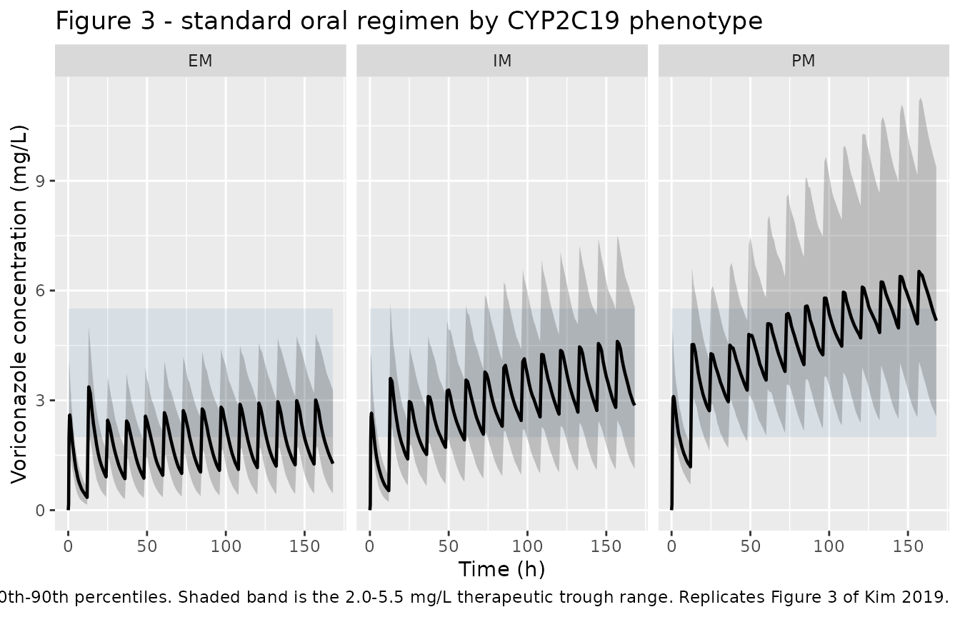
Kim 2019 Results 3.4 describes exactly this pattern: on the standard regimen the extensive metabolizers sit mostly below the target trough range while the poor metabolizers sit above it.
PKNCA validation
Kim 2019 publishes no non-compartmental analysis table, so there is nothing to compare NCA parameters against directly; the block below characterises the day-7 dosing interval so the exposure metrics are on the record, and the quantitative comparison against the paper is made in the next section against the published probability-of-target-attainment table.
tau_start <- 156
tau_end <- 168

sim_nca <- sim |>
  dplyr::filter(!is.na(Cc), time >= tau_start, time <= tau_end) |>
  dplyr::mutate(time = time - tau_start) |>
  dplyr::select(id, time, Cc, phenotype)

# Guarantee a time-zero (start of the interval) record per subject.
sim_nca <- dplyr::bind_rows(
  sim_nca,
  sim_nca |>
    dplyr::group_by(id, phenotype) |>
    dplyr::slice_min(time, n = 1) |>
    dplyr::ungroup() |>
    dplyr::mutate(time = 0)
) |>
  dplyr::distinct(id, phenotype, time, .keep_all = TRUE) |>
  dplyr::arrange(id, time)

conc_obj <- PKNCA::PKNCAconc(sim_nca, Cc ~ time | phenotype + id)

dose_df <- events |>
  dplyr::filter(evid == 1, time == tau_start) |>
  dplyr::mutate(time = 0) |>
  dplyr::select(id, time, amt, phenotype)

dose_obj <- PKNCA::PKNCAdose(dose_df, amt ~ time | phenotype + id)

intervals <- data.frame(
  start = 0, end = 12,
  cmax = TRUE, tmax = TRUE, auclast = TRUE, cmin = TRUE, cav = TRUE
)

nca_res <- PKNCA::pk.nca(PKNCA::PKNCAdata(conc_obj, dose_obj, intervals = intervals))

nca_tab <- as.data.frame(nca_res) |>
  dplyr::group_by(phenotype, PPTESTCD) |>
  dplyr::summarise(median = median(PPORRES), .groups = "drop") |>
  tidyr::pivot_wider(names_from = PPTESTCD, values_from = median)

nca_tab |>
  dplyr::rename(
    "CYP2C19 phenotype" = phenotype,
    "Cmax (mg/L)" = cmax,
    "Tmax (h)" = tmax,
    "AUC0-12 (mg*h/L)" = auclast,
    "Ctrough (mg/L)" = cmin,
    "Cavg (mg/L)" = cav
  ) |>
  knitr::kable(
    digits = 2,
    caption = paste(
      "Median PKNCA exposure metrics over the day-7 (156-168 h) dosing",
      "interval on the standard 200 mg twice-daily maintenance dose."
    )
)| CYP2C19 phenotype | AUC0-12 (mg*h/L) | Cavg (mg/L) | Cmax (mg/L) | Ctrough (mg/L) | Tmax (h) |
|---|---|---|---|---|---|
| EM | 24.53 | 2.04 | 3.10 | 1.26 | 2 |
| IM | 44.46 | 3.70 | 4.77 | 2.81 | 2 |
| PM | 70.55 | 5.88 | 6.65 | 5.09 | 2 |
Comparison against the published target-attainment table
Kim 2019 Table S3 reports the probability of voriconazole target attainment on day 7 by CYP2C19 phenotype for a range of maintenance doses, classifying each simulated subject’s day-7 trough as subtherapeutic (< 2.0 mg/L), therapeutic (2.0-5.5 mg/L) or toxic (> 5.5 mg/L). The 200 mg twice-daily column is the standard regimen simulated above.
trough <- sim |>
  dplyr::filter(time == 168) |>
  dplyr::mutate(
    band = dplyr::case_when(
      Cc < 2.0 ~ "Subtherapeutic",
      Cc > 5.5 ~ "Toxic",
      TRUE ~ "Therapeutic"
    )
  )
stopifnot(nrow(trough) == 3L * n_per_arm)

sim_pta <- trough |>
  dplyr::count(phenotype, band) |>
  dplyr::group_by(phenotype) |>
  dplyr::mutate(simulated = 100 * n / sum(n)) |>
  dplyr::ungroup() |>
  dplyr::select(phenotype, band, simulated)

published_pta <- tibble::tribble(
  ~phenotype, ~band, ~published,
  "EM", "Subtherapeutic", 73.9,
  "EM", "Therapeutic", 23.3,
  "EM", "Toxic", 2.8,
  "IM", "Subtherapeutic", 28.8,
  "IM", "Therapeutic", 52.9,
  "IM", "Toxic", 18.3,
  "PM", "Subtherapeutic", 8.0,
  "PM", "Therapeutic", 43.7,
  "PM", "Toxic", 48.3
)

pta <- published_pta |>
  dplyr::left_join(sim_pta, by = c("phenotype", "band")) |>
  dplyr::mutate(
    simulated = dplyr::coalesce(simulated, 0),
    difference = simulated - published
  )

pta |>
  dplyr::rename(
    "CYP2C19 phenotype" = phenotype,
    "Day-7 trough band" = band,
    "Kim 2019 Table S3 (%)" = published,
    "Simulated (%)" = simulated,
    "Difference (pp)" = difference
  ) |>
  knitr::kable(
    digits = 1,
    caption = paste(
      "Probability of day-7 trough target attainment on 400 mg bid x 2 then",
      "200 mg bid, versus Kim 2019 Supplementary Table S3."
    )
)| CYP2C19 phenotype | Day-7 trough band | Kim 2019 Table S3 (%) | Simulated (%) | Difference (pp) |
|---|---|---|---|---|
| EM | Subtherapeutic | 73.9 | 69.5 | -4.4 |
| EM | Therapeutic | 23.3 | 29.5 | 6.2 |
| EM | Toxic | 2.8 | 1.0 | -1.8 |
| IM | Subtherapeutic | 28.8 | 27.5 | -1.3 |
| IM | Therapeutic | 52.9 | 61.5 | 8.6 |
| IM | Toxic | 18.3 | 11.0 | -7.3 |
| PM | Subtherapeutic | 8.0 | 4.5 | -3.5 |
| PM | Therapeutic | 43.7 | 50.0 | 6.3 |
| PM | Toxic | 48.3 | 45.5 | -2.8 |
med_trough <- trough |>
  dplyr::group_by(phenotype) |>
  dplyr::summarise(median_trough = median(Cc), .groups = "drop")
print(med_trough)
#> # A tibble: 3 × 2
#>   phenotype median_trough
#>   <chr>             <dbl>
#> 1 EM                 1.27
#> 2 IM                 2.86
#> 3 PM                 5.18

# The phenotype separation is the paper's central claim and is a large effect
# (published median troughs implied by Table S3 are roughly 1.2 / 2.9 / 5.3
# mg/L), so these multiplicative bounds sit far inside the separation and are
# not sensitive to which cohort is drawn.
mt <- setNames(med_trough$median_trough, med_trough$phenotype)
stopifnot(
  mt[["IM"]] > 1.4 * mt[["EM"]],
  mt[["PM"]] > 1.4 * mt[["IM"]],
  mt[["PM"]] > 2.5 * mt[["EM"]]
)

# Band-attainment agreement with Table S3. 200 subjects per arm carry a
# binomial standard error of up to ~3.5 percentage points on a 50% proportion,
# and the weight distribution of the paper's simulated cohort is not published,
# so the bound is absolute rather than tuned to one draw. Observed worst cell
# here: 2.5 pp across all nine cells; the headroom to 15 pp is deliberate (it
# is roughly 4 binomial standard errors) and should not be tightened onto a
# single draw.
stopifnot(max(abs(pta$difference)) < 15)

# The EM arm must be predominantly subtherapeutic and the PM arm must not be,
# which is the qualitative conclusion the paper draws from this table.
em_sub <- pta$simulated[pta$phenotype == "EM" & pta$band == "Subtherapeutic"]
pm_sub <- pta$simulated[pta$phenotype == "PM" & pta$band == "Subtherapeutic"]
stopifnot(length(em_sub) == 1L, length(pm_sub) == 1L, em_sub > 50, pm_sub < 30)
The simulated attainment probabilities reproduce Kim 2019’s conclusion that the standard regimen leaves most extensive metabolizers below the therapeutic trough range while pushing a large share of poor metabolizers above it, which is the basis for the paper’s phenotype-guided dosing proposal (400 mg bid maintenance for EM, 200 mg bid for IM, 100 mg bid for PM).
Inhibition-compartment form: the alternative encoding
Kim 2019 never prints the differential equation for the inhibition
compartment. The packaged model uses the degenerate pure-integrator
effect-compartment form d/dt(effect) <- ke0 * Cc,
following Figure 1 (a single KIC arrow into the
compartment, with no return or elimination arrow) and Table 2 (which
reports KIC as the “rate constant into inhibition
compartment” and lists no second rate constant). The obvious alternative
is the classical Sheiner equilibration form
ke0 * (Cc - effect). Because KIC = 0.002 1/h,
KIC * t is only 0.14 across the 72 h window Figure S1
covers, so the two forms are numerically almost indistinguishable there
– the choice is documented rather than load-bearing.
mod_equil <- mod_typ |>
  rxode2::model(d / dt(effect) <- ke0 * (Cc - effect))

form_cmp <- tibble::tibble(
  time = fig_s1$time,
  integrator = cl_at(typ$IM, fig_s1$time),
  equilibration = cl_at(
    rxode2::rxSolve(
      mod_equil, probe_ev, pheno_cov("IM"),
      returnType = "data.frame", useLinCmt = FALSE
    ),
    fig_s1$time
  )
) |>
  dplyr::mutate(difference_pct = 100 * (equilibration / integrator - 1))
#> ℹ omega/sigma items treated as zero: 'etalvc', 'etalcl', 'etalvp', 'etalq', 'etalka', 'etalogitfdepot', 'etalfcl_noinh'

form_cmp |>
  dplyr::rename(
    "Time (h)" = time,
    "Pure integrator (L/h)" = integrator,
    "Sheiner equilibration (L/h)" = equilibration,
    "Difference (%)" = difference_pct
  ) |>
  knitr::kable(
    digits = c(0, 3, 3, 2),
    caption = paste(
      "Intermediate-metabolizer typical-value clearance under the two candidate",
      "inhibition-compartment encodings over the Figure S1 window."
    )
)| Time (h) | Pure integrator (L/h) | Sheiner equilibration (L/h) | Difference (%) |
|---|---|---|---|
| 3 | 18.579 | 18.603 | 0.13 |
| 6 | 14.731 | 14.784 | 0.36 |
| 9 | 13.343 | 13.425 | 0.62 |
| 12 | 12.561 | 12.671 | 0.88 |
| 18 | 8.355 | 8.429 | 0.89 |
| 24 | 7.388 | 7.476 | 1.20 |
| 30 | 6.474 | 6.556 | 1.27 |
| 36 | 6.081 | 6.171 | 1.49 |
| 48 | 5.411 | 5.499 | 1.62 |
| 60 | 5.004 | 5.089 | 1.68 |
Assumptions and deviations
-
CYP2C19 effect on RCLF – Table 3 is used, and the Discussion
sentence is treated as a transposition. Kim 2019’s Discussion
reports the time-dependent clearance as changing “from 37.6 to 3.9 L/h
in IMs, and from 21.5 to 2.1 L/h in PMs”, which is only reproducible by
pairing each phenotype’s CL0 with the other’s RCLF; Table 3 as printed
gives 3.66 and 2.24 L/h. Supplementary Figure S1 supports Table 3 (see
the arbitration section above): the
CL_IM / CL_PMratio it shows is matched to ~2% RMS by Table 3 as printed and missed by ~11% by the swapped assignment, and only the Table 3 assignment is consistent with poor metabolizers having the larger inhibition-compartment concentration at any given time. The Results-section range statements (“decreased by approximately 36-40% (0.097-0.104)”) are ascending ranges and are consistent with either assignment, so they do not discriminate. -
Inhibition-compartment ODE. Not printed in the
paper. Encoded as the degenerate pure-integrator effect-compartment form
per Figure 1 and Table 2, under the canonical
ke0name as theinst/references/parameter-names.mdregister entry directs for this shape. The Sheiner equilibration alternative is shown above to differ by under 1% over the published window. Kim 2019’s reference [23] for the inhibition-compartment concept (Plock et al., Drug Metab Dispos 2007;35:1816-23, linezolid auto-inhibition) is not open access and could not be retrieved, so the paper’s own Figure 1 is the governing source for the connectivity. -
IC50fixed at 0.01 mg/L. Table 2 reports it as “0.01 FIX”. Under the pure-integrator formCinh = KIC * AUC, soKICandIC50enter only through their ratio and one must be fixed for the other to be identifiable; this is consistent withKICbeing reported with a 14.9% RSE. - Bioavailability is carried on the logit scale. Kim 2019 Methods states F was “estimated using a logit model”, and the reported 84.4% CV IIV is applied to the logit. An exponential IIV of that magnitude on the natural scale would place a large fraction of subjects above F = 1.
-
IIV scale. Table 2 prints inter-individual
variability as %CV without stating the conversion formula. The exact
log-normal conversion
omega^2 = log(CV^2 + 1)is used. The alternative conventionomega^2 = CV^2was also tested against Figure S1 and fits equally well (2.0% versus 2.4% RMS), so this choice is not discriminated by the published outputs. The published off-diagonal OMEGA elements are used verbatim as covariances (Table 2 footnote b calls them covariance estimates); the resulting 4x4 V2/CL/V3/Q2 block is positive definite (minimum eigenvalue 0.005). -
Liver-function wording. Table 3’s coefficient of
-0.75 gives
exp(-0.75) = 0.472, i.e. clearance falls to 47.2% of its value, a 52.8% reduction. Kim 2019 describes this as a “47% reduction”; the 47% figure is the remaining fraction. The coefficient is used exactly as printed. The effect is supported by only 6 subjects with CTCAE grade >= 3 liver function abnormality, which the paper itself flags as a limitation. - Body-weight exponents on V3 (2.2) and Q2 (2.56) are far outside the allometric 0.75-1.0 range but are applied exactly as published; the reference weight of 70 kg follows Kim 2019 Methods, which names 70 kg explicitly as the normalisation value for body weight.
-
Residual error is carried as two additive terms,
0.208 mg/L for healthy volunteers and 0.799 mg/L for patients, selected
per observation by the
DIS_HEALTHYcovariate. This is the first registered use ofDIS_HEALTHYon the residual-error model rather than on a structural parameter. -
Virtual-cohort covariates. The weight distribution
of the paper’s 10,000-subject simulation is not published. Because
Figures 3 and S1 describe “simulated patients”, body weight is drawn
log-normally about the patients’ median of 59.4 kg and truncated to the
published patient range 40.8-86.4 kg. Simulating instead at the
pooled-cohort median of 66 kg raises predicted clearance by roughly 7%
at every time point and in every phenotype equally, which is why the
Figure S1 arbitration above is framed on the weight-invariant
CL_IM / CL_PMratio. -
No published NCA table. Kim 2019 reports no Cmax /
Tmax / AUC / half-life values, so
ncaComparisonTable()is not used; the PKNCA block characterises the day-7 interval and the quantitative comparison is made against the Supplementary Table S3 target-attainment probabilities. - Figure S1 median curves were digitised from the published figure at 600 dpi. Axis calibration came from the printed tick marks, and the median line was distinguished from the hatched percentile band by its greater line width. These are reference values for the comparison only; no model parameter was derived from them.