Copanlisib in children and adolescents (Morcos 2023b)
Source:vignettes/articles/Morcos_2023b_copanlisib.Rmd
Morcos_2023b_copanlisib.RmdModel and source
#> ℹ parameter labels from comments will be replaced by 'label()'Citation: Morcos PN, Schlender J, Burghaus R, Moss J, Lloyd A, Childs BH, Macy ME, Reid JM, Chung J, Garmann D. Model-informed approach to support pediatric dosing for the pan-PI3K inhibitor copanlisib in children and adolescents with relapsed/refractory solid tumors. Clin Transl Sci. 2023;16(7):1197-1209. doi:10.1111/cts.13523. Adult backbone parameters: Morcos PN, Moss J, Austin R, Hiemeyer F, Zinzani PL, Beckert V, Mongay Soler L, Childs BH, Garmann D. Copanlisib population pharmacokinetics from phase I-III studies and exposure-response relationships in combination with rituximab. CPT Pharmacometrics Syst Pharmacol. 2023;12(11):1666-1686. doi:10.1002/psp4.13000.
Description: Three-compartment population PK model for intravenous copanlisib adapted from the adult phase I-III model to children and adolescents (4-21 years) with relapsed/refractory solid tumors: every clearance and volume is scaled by body surface area relative to 1.88 m^2 with a fixed exponent of 1, with the adult typical values, categorical covariate effects (rifampicin and itraconazole comedication, sex, hepatic impairment, Japanese region, CHRONOS-3 study membership), IIV and infusion-time / study-phase stratified log-additive residual error carried over unchanged
Article: https://doi.org/10.1111/cts.13523 (open access)
Adult backbone: https://doi.org/10.1002/psp4.13000, packaged as
Morcos_2023_copanlisib(see the Copanlisib (Morcos 2023) article)
Copanlisib is an intravenous pan-class-I PI3K inhibitor. Morcos 2023 (Clin Transl Sci) supported the starting dose of 28 mg/m^2 for a pediatric phase I study (Bayer study 19176) with two models:
- An adult whole-body PBPK model built in PK-Sim (Open Systems Pharmacology Suite 6.0), extended to children through PK-Sim’s built-in age-dependent physiology. It is not packaged; see Assumptions and deviations.
- The adult population PK model, adapted to children by scaling every
clearance and volume by body surface area:
P = P_adult * (BSA / 1.88)^1. The adapted model was not re-estimated. It was used as is to estimate individual exposure from the pediatric samples and to simulate a virtual pediatric population. This is the packaged model.
The adult model cited by the pediatric paper (its reference 9, a 2022 AACR poster) is the analysis published in full as Morcos 2023 CPT:PSP. That paper’s figures are credited as “previously presented in a poster at the Third AACR International Meeting … June 23-26, 2022”, which is the poster the pediatric paper cites. Every typical value, covariate effect, IIV and residual magnitude therefore comes from Morcos 2023 CPT:PSP Table 2. The pediatric paper adds only the BSA term.
Population
| Field | Value |
|---|---|
| species | human |
| n_subjects | 30 |
| n_studies | 1 |
| n_observations | 160 |
| age_range | 4-21 years |
| age_median | 13 years |
| bsa_range | 0.64-2.44 m^2 |
| bsa_median | 1.37 m^2 |
| disease_state | children and adolescents with relapsed/refractory solid tumors or lymphoma for which there is no standard curative treatment |
| dose_range | 28 mg/m2 (n = 24) or 35 mg/m2 (n = 7) as an intravenous infusion on days 1, 8 and 15 of a 28-day cycle |
| notes | Morcos 2023 CTS Results, ‘PopPK modeling’: 31 pediatric patients in the open-label phase I dose-escalation study 19176 (Rolling-6 design) gave 191 samples; 30 pre-dose BLQ samples and 1 kinetically implausible sample were removed, leaving 160 observations in 30 patients. Samples were drawn pre-infusion, at 1-1.25 h, 1.5-3 h (age >= 6 years only) and 22-24 h after the start of the infusion on cycle 1 days 1 and 15; LC/MS LLOQ 0.5 ng/mL. The pediatric data were used only to evaluate the adapted model: no parameter was re-estimated. Every typical value, covariate effect, IIV and residual magnitude below is the adult estimate of Morcos 2023 CPT:PSP (712 adults, nine phase I-III studies). The sex split of the pediatric cohort is not reported. |
Thirty-one children and adolescents with relapsed or refractory solid tumors or lymphoma were enrolled in the Rolling-6 dose escalation. Twenty-four received 28 mg/m^2 and seven received 35 mg/m^2 on days 1, 8 and 15 of a 28-day cycle. After removing 30 pre-dose BLQ samples and one implausible sample, 160 concentrations from 30 patients remained. Their median age was 13 years (range 4-21) and median BSA 1.37 m^2 (range 0.64-2.44). The paper does not report the cohort’s sex split, hepatic function or enrollment region.
Source trace
| Equation / parameter | Value | Source location |
|---|---|---|
| Three-compartment IV disposition, first-order elimination from central | n/a | Morcos 2023 CPT:PSP Results, “PopPK meta-analyses”; Figure S1 |
| BSA power scaling on CL, V1, Q2, V2, Q3, V3, centred on 1.88 m^2 | n/a | Morcos 2023 CTS Methods, “Population PK modeling” |
e_bsa_cl, e_bsa_vc, e_bsa_q,
e_bsa_vp, e_bsa_q2,
e_bsa_vp2
|
1 (fixed) | Morcos 2023 CTS Methods: “an exponent of 1 on all rate (including clearance) and volume parameters”; Results: alternatives “did not offer significant improvement” |
| No re-estimation of adult parameters | n/a | Morcos 2023 CTS Methods: “used without further modification or any parameter re-estimation” |
lcl (CL) |
22.2 L/h | Morcos 2023 CPT:PSP Table 2, CL pop
|
lvc (V1) |
92.1 L | Morcos 2023 CPT:PSP Table 2, V1 pop
|
lq (Q2) |
79.3 L/h | Morcos 2023 CPT:PSP Table 2, Q2
|
lvp (V2) |
508 L | Morcos 2023 CPT:PSP Table 2, V2
|
lq2 (Q3) |
7.34 L/h | Morcos 2023 CPT:PSP Table 2, Q3
|
lvp2 (V3) |
522 L | Morcos 2023 CPT:PSP Table 2, V3
|
e_conmed_rifampicin_cl /
e_conmed_rifampicin_vc
|
1.91 / 1.08 | Morcos 2023 CPT:PSP Table 2 Theta RIFCL /
Theta RIFV1
|
e_conmed_itraconazole_cl |
-0.361 | Morcos 2023 CPT:PSP Table 2 Theta ITRACL
|
e_study_chronos3_cl |
-0.184 | Morcos 2023 CPT:PSP Table 2 Theta 17067CL
|
e_sexf_cl / e_sexf_vc
|
-0.167 / -0.429 | Morcos 2023 CPT:PSP Table 2 Theta SEXCL /
Theta SEXV1
|
e_hepimp_cl |
-0.192 | Morcos 2023 CPT:PSP Table 2 Theta NCICL
|
e_region_japan_cl |
-0.204 | Morcos 2023 CPT:PSP Table 2 Theta JAPCL
|
etalcl / etalvc variances |
0.124 / 0.846 | Morcos 2023 CPT:PSP Table 2 OMEGA (CV 36.3% / 115%) |
expSd_early / expSd_phase12 /
expSd_phase3
|
sqrt(5.10) / sqrt(0.176) / sqrt(0.632) | Morcos 2023 CPT:PSP Table 2 SIGMA and footnote g (log-additive) |
The adaptation reduces exactly to the adult model at 1.88 m^2
With BSA = 1.88 m^2, every scaling factor is 1, so the packaged
pediatric model must reproduce the packaged adult model exactly. At any
other BSA, CL and V1 must scale by exactly BSA / 1.88. Both
are deterministic identities (the same parameters on both sides, typical
values only), so they are asserted tightly.
mod      <- readModelDb("Morcos_2023b_copanlisib")
mod_typ  <- rxode2::zeroRe(mod)
#> ℹ parameter labels from comments will be replaced by 'label()'
#> Warning: No sigma parameters in the model
adult_typ <- rxode2::zeroRe(readModelDb("Morcos_2023_copanlisib"))
#> ℹ parameter labels from comments will be replaced by 'label()'
#> Warning: No sigma parameters in the model

cov_zero <- c(CONMED_RIFAMPICIN = 0, CONMED_ITRACONAZOLE = 0, STUDY_CHRONOS3 = 0,
              HEPIMP = 0, REGION_JAPAN = 0)

# Two subjects (male, female); 60 mg over 1 h into `central`, observations on
# the ODE state.
probe_ev <- bind_rows(
  tibble::tibble(id = 1:2, time = 0, amt = 60, rate = 60, evid = 1L),
  tidyr::expand_grid(id = 1:2, time = c(0.5, 1, 2, 24, 168)) |>
    mutate(amt = NA_real_, rate = NA_real_, evid = 0L)
) |>
  mutate(cmt = "central", SEXF = id - 1) |>
  bind_cols(tibble::as_tibble(as.list(cov_zero))) |>
  arrange(id, time, desc(evid))

sim_adult <- rxode2::rxSolve(adult_typ, events = probe_ev) |> as.data.frame()
#> ℹ omega/sigma items treated as zero: 'etalcl', 'etalvc'
#> Warning: multi-subject simulation without without 'omega'
sim_ref   <- rxode2::rxSolve(mod_typ, events = mutate(probe_ev, BSA = 1.88)) |> as.data.frame()
#> ℹ omega/sigma items treated as zero: 'etalcl', 'etalvc'
#> Warning: multi-subject simulation without without 'omega'
sim_small <- rxode2::rxSolve(mod_typ, events = mutate(probe_ev, BSA = 0.94)) |> as.data.frame()
#> ℹ omega/sigma items treated as zero: 'etalcl', 'etalvc'
#> Warning: multi-subject simulation without without 'omega'

identity_tbl <- tibble::tibble(
  Check = c("Cc, pediatric model at 1.88 m^2 vs adult model (max rel. diff)",
            "CL ratio at 0.94 m^2 vs 1.88 m^2 (expected 0.5)",
            "V1 ratio at 0.94 m^2 vs 1.88 m^2 (expected 0.5)"),
  Value = c(max(abs(sim_ref$Cc / sim_adult$Cc - 1)),
            unique(round(sim_small$cl / sim_ref$cl, 12)),
            unique(round(sim_small$vc / sim_ref$vc, 12)))
)
knitr::kable(identity_tbl, digits = 12)| Check | Value |
|---|---|
| Cc, pediatric model at 1.88 m^2 vs adult model (max rel. diff) | 0.0 |
| CL ratio at 0.94 m^2 vs 1.88 m^2 (expected 0.5) | 0.5 |
| V1 ratio at 0.94 m^2 vs 1.88 m^2 (expected 0.5) | 0.5 |
stopifnot(
  max(abs(sim_ref$Cc / sim_adult$Cc - 1)) < 1e-8,
  isTRUE(all.equal(sim_small$cl / sim_ref$cl, rep(0.5, nrow(sim_ref)))),
  isTRUE(all.equal(sim_small$vc / sim_ref$vc, rep(0.5, nrow(sim_ref))))
)
Because every clearance and volume scales with the same power of BSA,
the rate constants (CL/V1, Q2/V1,
Q2/V2, …) do not depend on BSA at all. With a dose in
mg/m^2, the amount given and every volume scale together, so the
typical concentration-time profile does not depend on
BSA. That is the mechanism behind the paper’s finding of
“uniform copanlisib exposures across the investigated pediatric age
range”. It also means the BSA distribution of the virtual cohort below
cannot move the exposure distribution; only sex and the random effects
can.
bsa_grid <- c(0.64, 1.00, 1.37, 1.88, 2.44)
inv_ev <- tidyr::expand_grid(BSA = bsa_grid, time = c(0, 0.5, 1, 2, 24, 168)) |>
  mutate(id = match(BSA, bsa_grid))
inv_ev <- bind_rows(
  inv_ev |> distinct(id, BSA) |>
    mutate(time = 0, amt = 28 * BSA, rate = 28 * BSA, evid = 1L),
  inv_ev |> mutate(amt = NA_real_, rate = NA_real_, evid = 0L)
) |>
  mutate(cmt = "central", SEXF = 0) |>
  bind_cols(tibble::as_tibble(as.list(cov_zero))) |>
  arrange(id, time, desc(evid))

sim_inv <- rxode2::rxSolve(mod_typ, events = inv_ev) |> as.data.frame()
#> ℹ omega/sigma items treated as zero: 'etalcl', 'etalvc'
#> Warning: multi-subject simulation without without 'omega'
inv_spread <- sim_inv |>
  filter(time > 0) |>
  group_by(time) |>
  summarise(rel_spread = (max(Cc) - min(Cc)) / mean(Cc), .groups = "drop")
knitr::kable(inv_spread, digits = 12,
caption = "Relative spread of typical Cc across BSA 0.64-2.44 m^2 at 28 mg/m^2 (male reference patient).")| time | rel_spread |
|---|---|
| 0.5 | 3.43300e-09 |
| 1.0 | 1.49000e-08 |
| 2.0 | 1.78730e-08 |
| 24.0 | 2.36320e-08 |
| 168.0 | 5.17894e-07 |
Virtual cohort
Morcos 2023 CTS Figure 5 simulates 500 virtual patients per year of age from 4 to 21 years (250 male, 250 female) with BSA sampled from NHANES III, given 28 mg/m^2 on days 1, 8 and 15. NHANES III is not distributed with this package, so BSA for age comes from CDC 50th-percentile weight and stature (averaged across sexes) with lognormal scatter, via the Mosteller formula. As shown above, the choice cannot change the AUC distribution. To keep the article fast, the cohort has 10 patients per year of age (5 male, 5 female), 180 in all.
The adult comparator is CHRONOS-1 (study 16349 part B, the
monotherapy pivotal study, 60 mg flat). Its demographics come from the
Study 16349 (Part B) row of Morcos 2023 CPT:PSP Table 1:
122 patients, 48.4% female, 9.0% with mild hepatic impairment. Adults
are simulated at BSA = 1.88 m^2, where the adapted model is the adult
model.
rxode2::rxSetSeed(20231197)
set.seed(20231197)

growth <- tibble::tribble(
  ~age,  ~wt,  ~ht,
  4.00,  16.3, 102,
  5.00,  18.3, 109,
  6.00,  20.6, 115,
  7.00,  23.0, 121,
  8.00,  25.6, 127,
  10.00, 32.0, 138,
  12.00, 40.5, 149,
  14.00, 50.0, 162,
  16.00, 58.0, 168,
  18.00, 63.0, 170,
  21.00, 68.0, 171
)

n_per_age <- 10L
peds <- tidyr::expand_grid(AGE = 4:21, k = seq_len(n_per_age)) |>
  mutate(
    SEXF   = as.numeric(k > n_per_age / 2),
    wt_med = stats::approx(growth$age, growth$wt, xout = AGE)$y,
    ht_med = stats::approx(growth$age, growth$ht, xout = AGE)$y,
    WT     = wt_med * exp(stats::rnorm(n(), 0, 0.20)),
    HT     = ht_med * exp(stats::rnorm(n(), 0, 0.045)),
    BSA    = sqrt(HT * WT / 3600),
    dose   = 28 * BSA,
    HEPIMP = 0,
    arm    = "Pediatric 28 mg/m2"
  )

n_adult <- 200L
adults <- tibble::tibble(
  AGE    = NA_real_,
  SEXF   = as.numeric(stats::runif(n_adult) < 0.484),
  HEPIMP = as.numeric(stats::runif(n_adult) < 0.090),
  BSA    = 1.88,
  dose   = 60,
  arm    = "Adult CHRONOS-1 60 mg"
)

cohort <- bind_rows(peds, adults) |>
  mutate(id = seq_len(n()), CONMED_RIFAMPICIN = 0, CONMED_ITRACONAZOLE = 0,
         STUDY_CHRONOS3 = 0, REGION_JAPAN = 0) |>
  select(id, arm, AGE, SEXF, HEPIMP, BSA, dose, CONMED_RIFAMPICIN,
         CONMED_ITRACONAZOLE, STUDY_CHRONOS3, REGION_JAPAN)

cohort |>
  group_by(arm) |>
  summarise(
    N = n(),
    `Female (%)` = 100 * mean(SEXF),
    `BSA median (range), m^2` = sprintf("%.2f (%.2f-%.2f)", median(BSA), min(BSA), max(BSA)),
    .groups = "drop"
  ) |>
knitr::kable(caption = "Virtual cohort.")| arm | N | Female (%) | BSA median (range), m^2 |
|---|---|---|---|
| Adult CHRONOS-1 60 mg | 200 | 51 | 1.88 (1.88-1.88) |
| Pediatric 28 mg/m2 | 180 | 50 | 1.36 (0.58-2.40) |
Simulation
Three 1-h infusions one week apart (days 1, 8 and 15). AUC(0-168)nd, the exposure metric of both papers, is the AUC over the week after the third nominal dose, i.e. from 336 to 504 h.
auc_start <- 336
auc_end   <- 504
obs_times <- sort(unique(c(0, auc_start + c(0, seq(0.25, 4, by = 0.25),
                                            seq(5, 24, by = 1),
                                            seq(28, 168, by = 4)))))

dose_rows <- tidyr::expand_grid(cohort, time = c(0, 168, 336)) |>
  mutate(amt = dose, rate = dose, evid = 1L)
obs_rows <- tidyr::expand_grid(cohort, time = obs_times) |>
  mutate(amt = NA_real_, rate = NA_real_, evid = 0L)
events <- bind_rows(dose_rows, obs_rows) |>
  mutate(cmt = "central") |>
  arrange(id, time, desc(evid))

sim <- rxode2::rxSolve(mod, events = events, keep = c("arm", "AGE")) |>
  as.data.frame()
#> ℹ parameter labels from comments will be replaced by 'label()'
PKNCA validation
sim_nca <- sim |>
  filter(!is.na(Cc)) |>
  select(id, time, Cc, arm)

# The observation grid already contains time 0 (pre-dose, 0 mg/L) for every
# subject; assert it rather than re-adding it.
stopifnot(all(tapply(sim_nca$time == 0, sim_nca$id, any)))

conc_obj <- PKNCA::PKNCAconc(as.data.frame(sim_nca), Cc ~ time | arm + id,
                             concu = "mg/L", timeu = "h")
dose_obj <- PKNCA::PKNCAdose(
  as.data.frame(filter(events, evid == 1L) |> select(id, time, amt, arm)),
  amt ~ time | arm + id, doseu = "mg"
)
intervals <- data.frame(start = auc_start, end = auc_end,
                        cmax = TRUE, auclast = TRUE)

nca_res <- PKNCA::pk.nca(PKNCA::PKNCAdata(conc_obj, dose_obj, intervals = intervals))

auc_ind <- as.data.frame(nca_res$result) |>
  filter(PPTESTCD == "auclast") |>
  select(id, arm, auclast = PPORRES) |>
  mutate(auc_ug = 1000 * auclast) |>
  left_join(distinct(cohort, id, AGE), by = "id")
Comparison against published exposure
Morcos 2023 CTS reports these exposures only graphically. The values below were digitised by the maintainers from Figure 5: the pediatric simulated median (about 2600 ugh/L) and 90% prediction interval (about 1450-4500 ugh/L), and the CHRONOS-1 observed median (about 2870 ugh/L) and 5th-95th percentiles (about 2100-4550 ugh/L).
published <- tibble::tibble(
  arm     = c("Pediatric 28 mg/m2", "Adult CHRONOS-1 60 mg"),
  auclast = c(2.600, 2.870)   # ug*h/L digitised from Figure 5, in mg*h/L
)

cmp <- nlmixr2lib::ncaComparisonTable(
  simulated     = nca_res,
  reference     = published,
  by            = "arm",
  params        = "auclast",
  units         = c(auclast = "mg*h/L"),
  tolerance_pct = 20
)
knitr::kable(cmp, caption = "Simulated median AUC(0-168)nd vs. Morcos 2023 CTS Figure 5 (digitised). * differs from reference by >20%.")| NCA parameter | arm | Reference | Simulated | % diff |
|---|---|---|---|---|
| AUClast (mg*h/L) | Pediatric 28 mg/m2 | 2.6 | 2.56 | -1.7% |
| AUClast (mg*h/L) | Adult CHRONOS-1 60 mg | 2.87 | 3.04 | +6.0% |
auc_summary <- auc_ind |>
  group_by(arm) |>
  summarise(
    Q05 = quantile(auc_ug, 0.05), Q50 = median(auc_ug), Q95 = quantile(auc_ug, 0.95),
    .groups = "drop"
  )
knitr::kable(auc_summary, digits = 0,
caption = "Simulated AUC(0-168)nd percentiles (ug*h/L).")| arm | Q05 | Q50 | Q95 |
|---|---|---|---|
| Adult CHRONOS-1 60 mg | 1755 | 3041 | 5243 |
| Pediatric 28 mg/m2 | 1349 | 2556 | 4883 |
ped <- auc_summary[auc_summary$arm == "Pediatric 28 mg/m2", ]
adu <- auc_summary[auc_summary$arm == "Adult CHRONOS-1 60 mg", ]

stopifnot(
  # Structural: a mis-transcribed clearance, sex effect or BSA centring value
  # moves the whole pediatric distribution by tens of percent.
  abs(ped$Q50 / 2600 - 1) < 0.10,
  # The adult comparator: CHRONOS-1 is printed as empirical-Bayes estimates,
  # which shrink towards the mean, so only the centre is compared.
  abs(adu$Q50 / 2870 - 1) < 0.15,
  # Envelope: the 90% interval spans a factor of about 3.1 in Figure 5
  # (4500 / 1450); this checks the IIV on CL is in the right range.
  (ped$Q95 / ped$Q05) > 2, (ped$Q95 / ped$Q05) < 4.5
)
The simulated pediatric distribution matches Figure 5. The paper
attributes the lower pediatric median to the dose: 28 mg/m^2 is 80% of
the adult 60 mg dose adjusted for BSA. For typical patients of the same
sex, the pediatric-to-adult AUC ratio is 28 * 1.88 / 60 =
0.877, whatever the child’s BSA. The paper also gives a geometric mean
ratio of 101% for the model-predicted individual AUC of the
enrolled pediatric patients against CHRONOS-1. Those are empirical-Bayes
estimates from the 30 real patients and cannot be reproduced without
their data; they suggest the enrolled children had somewhat lower
clearance than the typical value.
gmr <- exp(mean(log(auc_ind$auc_ug[auc_ind$arm == "Pediatric 28 mg/m2"]))) /
  exp(mean(log(auc_ind$auc_ug[auc_ind$arm == "Adult CHRONOS-1 60 mg"])))
knitr::kable(tibble::tibble(
  Quantity = c("Simulated pediatric / adult geometric mean AUC ratio",
               "Typical-value ratio 28 * 1.88 / 60",
               "Figure 5 simulated pediatric median / CHRONOS-1 observed median (digitised)",
               "Paper: enrolled pediatric (individual estimates) vs CHRONOS-1 GMR"),
  Value = c(gmr, 28 * 1.88 / 60, 2600 / 2870, 1.01)
), digits = 3)| Quantity | Value |
|---|---|
| Simulated pediatric / adult geometric mean AUC ratio | 0.814 |
| Typical-value ratio 28 * 1.88 / 60 | 0.877 |
| Figure 5 simulated pediatric median / CHRONOS-1 observed median (digitised) | 0.906 |
| Paper: enrolled pediatric (individual estimates) vs CHRONOS-1 GMR | 1.010 |
Replicates Figure 5 of Morcos 2023 CTS
ped_band <- auc_ind |>
  filter(arm == "Pediatric 28 mg/m2") |>
  summarise(Q05 = quantile(auc_ug, 0.05), Q50 = median(auc_ug),
            Q95 = quantile(auc_ug, 0.95))

auc_ind |>
  filter(arm == "Pediatric 28 mg/m2") |>
  ggplot(aes(AGE, auc_ug)) +
  annotate("rect", xmin = 3.5, xmax = 21.5, ymin = ped_band$Q05, ymax = ped_band$Q95,
           fill = "pink", alpha = 0.5) +
  geom_hline(yintercept = ped_band$Q50, colour = "red") +
  geom_jitter(width = 0.15, height = 0, shape = 1, colour = "darkred") +
  coord_cartesian(ylim = c(0, 9000)) +
  labs(x = "Age (years)", y = "AUC(0-168)nd (ug*h/L)",
       title = "Simulated AUC(0-168)nd after three weekly doses of 28 mg/m^2",
       caption = "Median (line) and 90% prediction interval (band). Replicates the left panel of Figure 5 of Morcos 2023 CTS.") +
  theme_bw()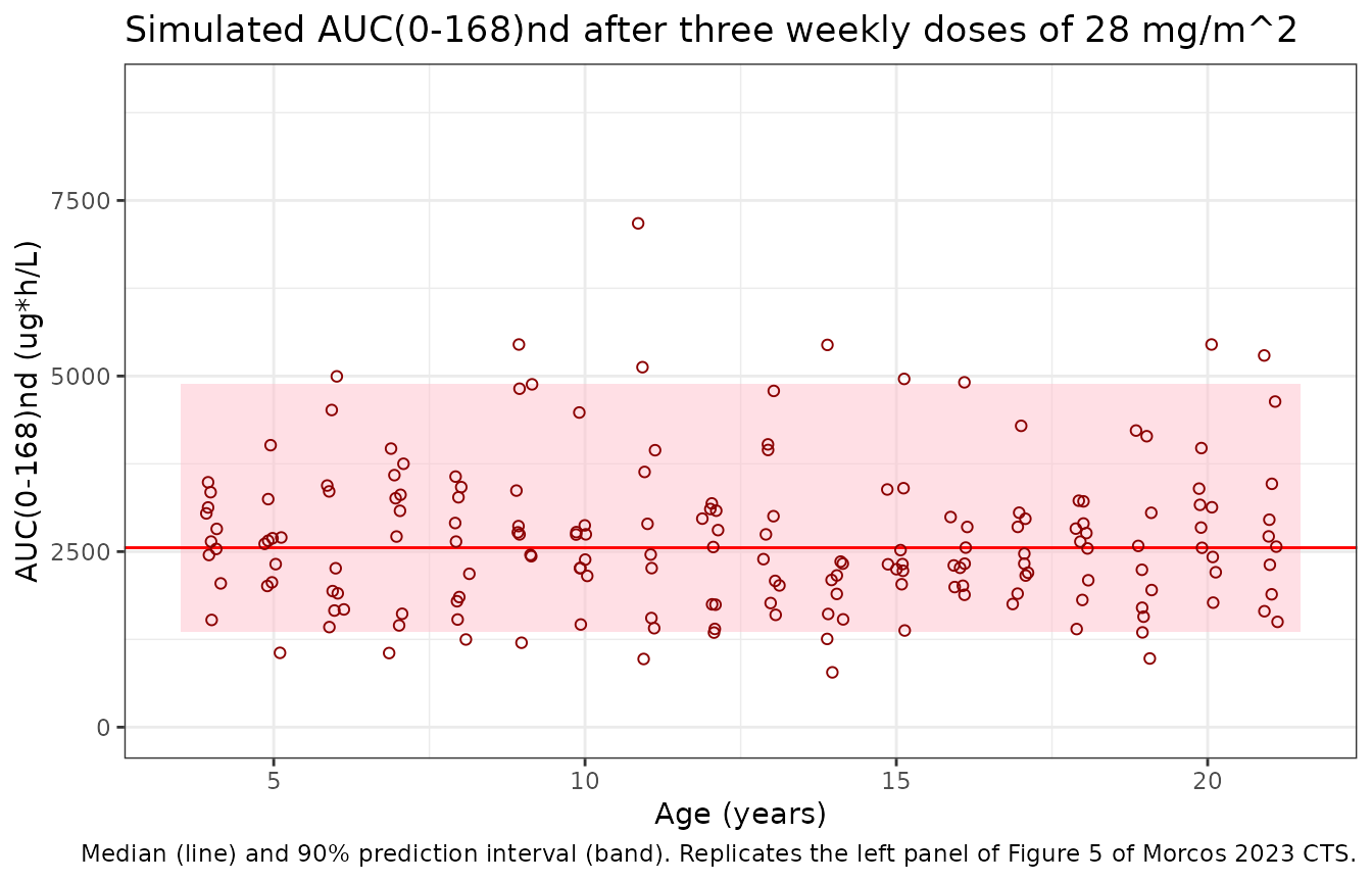
# Figure 5: exposure is flat across age. Medians by age band, robust to which
# subjects land in the tails.
age_bands <- auc_ind |>
  filter(arm == "Pediatric 28 mg/m2") |>
  mutate(band = cut(AGE, c(3, 8, 13, 17, 21), labels = c("4-8", "9-13", "14-17", "18-21"))) |>
  group_by(band) |>
  summarise(n = n(), median_auc = median(auc_ug), .groups = "drop")
knitr::kable(age_bands, digits = 0, caption = "Median simulated AUC(0-168)nd by age band (ug*h/L).")| band | n | median_auc |
|---|---|---|
| 4-8 | 50 | 2649 |
| 9-13 | 50 | 2745 |
| 14-17 | 40 | 2311 |
| 18-21 | 40 | 2612 |
Concentration-time profile after the third dose
sim |>
  filter(time >= auc_start) |>
  mutate(tad = time - auc_start) |>
  filter(tad > 0) |>
  group_by(arm, tad) |>
  summarise(Q05 = quantile(Cc, 0.05), Q50 = median(Cc), Q95 = quantile(Cc, 0.95),
            .groups = "drop") |>
  ggplot(aes(tad, 1000 * Q50, colour = arm, fill = arm)) +
  geom_ribbon(aes(ymin = 1000 * Q05, ymax = 1000 * Q95), alpha = 0.2, colour = NA) +
  geom_line() +
  scale_y_log10() +
  scale_x_continuous(breaks = seq(0, 168, by = 24)) +
  labs(x = "Time after third dose (h)", y = "Copanlisib (ug/L)", colour = NULL, fill = NULL,
       caption = "Median and 5th-95th percentiles.") +
  theme_bw() +
  theme(legend.position = "bottom")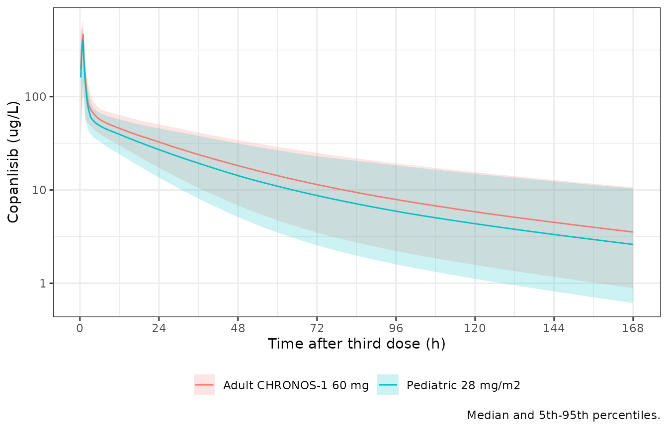
Assumptions and deviations
- The PBPK model is not packaged. The adult and pediatric PBPK models were built in PK-Sim. The paper prints only the drug-specific inputs (Table 1: physicochemistry, a hypothetical binding partner, P-gp and CYP3A4 kinetics). The organ volumes, blood flows, partition coefficients, expression profiles and ontogeny functions are outputs of the PK-Sim database and are not published, so the model cannot be reconstructed from the paper.
- The adult backbone comes from a second paper. The pediatric paper prints no adult parameter values. It cites a 2022 AACR poster, and Morcos 2023 CPT:PSP reproduces that poster’s figures. All values here are from Morcos 2023 CPT:PSP Table 2.
- All adult covariates are kept. The paper states the adult model was used “without further modification”, so the sex, hepatic-impairment, Japan, CHRONOS-3 and comedication effects remain. For the pediatric study the DDI, CHRONOS-3 and Japan indicators are 0. The paper does not report the cohort’s sex split, hepatic function or region, so the virtual cohort is half female (as in Figure 5) with normal hepatic function.
-
Residual error. The pediatric study is a phase I
study, so its samples beyond the first 20 min of an infusion use the
phase I/II residual stratum (
STUDY_CHRONOS3 = 0). - BSA source. Figure 5 sampled BSA from NHANES III, which is not available here. CDC growth medians with lognormal scatter and the Mosteller formula are used instead. The paper does not say which BSA formula it used. Under BSA^1 scaling with mg/m^2 dosing, the BSA values cannot affect the simulated AUC (shown above).
- Adult comparator. CHRONOS-1 is simulated at BSA = 1.88 m^2, where the adapted model equals the adult model, with 48.4% female and 9.0% mild hepatic impairment (Morcos 2023 CPT:PSP Table 1, study 16349 part B). The Japan column of that row reads as 0 Japanese patients and is set to 0. Figure 5 plots the CHRONOS-1 values as individual model-predicted (empirical-Bayes) exposures, which are shrunk towards the mean. The simulated adult tails are therefore wider than the published 5th-95th percentiles, and only the medians are compared.
- Figure values are digitised. The Figure 5 medians and intervals were read off the published figure by the maintainers and are accurate to about +/-100 ug*h/L.
- Cohort size. 10 virtual patients per year of age (180 in all) instead of 500, to keep the article fast.