MK-ASODN nanoliposomes, monkey and human PBPK (Bai 2021)
Source:vignettes/articles/Bai_2021_mkAsodnLiposome_pbpk.Rmd
Bai_2021_mkAsodnLiposome_pbpk.RmdModel and source
- Citation: Bai H, Cheng Y, Che J. Pharmacokinetics and Disposition of Heparin-Binding Growth Factor Midkine Antisense Oligonucleotide Nanoliposomes in Experimental Animal Species and Prediction of Human Pharmacokinetics Using a Physiologically Based Pharmacokinetic Model. Front Pharmacol. 2021;12:769538. doi:10.3389/fphar.2021.769538. PMCID PMC8595129. The human PBPK method, allometric equation and 90 mg dose derivation are Methods 2.7; human CL and Vss are Results 3.6; predicted human Cmax and AUC0-inf are Table 4; the simulated human plasma profile is Figure 3.
- Article: https://doi.org/10.3389/fphar.2021.769538
Monkey model:
Preclinical (macaque monkey). PBPK-derived reduced one-compartment intravenous model for MK-ASODN nanoliposomes, a nanoliposome-encapsulated 20-mer antisense oligonucleotide (5’-CCCCGGGCCGCCCTTCTTCA, 6044.4 Da) against midkine mRNA, developed for hepatocellular carcinoma. The source paper built a 14-tissue perfusion-limited whole-body PBPK model in GastroPlus 8.0 using the software’s default monkey physiology and Rodgers-Single (Lukacova) tissue-to-plasma partition coefficients; those organ volumes, blood flows and Kp values are platform internals that the publication does not print, so the whole-body structure is not reproduced here. What this file encodes is the plasma-level behaviour of that model: a single linear clearance of 0.1002 L/h/kg, which reproduces the paper’s own predicted AUC0-inf on all three dose arms (11.5, 23, 46 mg/kg) to four significant figures, and a volume of 0.1326 L/kg from the terminal slope of the simulated curves in Figure 1, whose back-extrapolated intercept reproduces the paper’s own tabulated predicted Cmax. The PBPK curve has a brief initial spike (under about 10 minutes) that a one-compartment reduction does not carry; the spike holds under 2% of the AUC. The PBPK model is linear, so it does not carry the less-than-dose-proportional exposure the observed monkey NCA showed. Clearance and volume scale linearly with body weight because the paper reports them per kg. The paper reports no interindividual or residual variability for the simulation, so no etas are declared and both residual error terms are fixed(0).
Human model:
PBPK-derived reduced one-compartment intravenous model for MK-ASODN nanoliposomes (a nanoliposome-encapsulated antisense oligonucleotide against midkine mRNA, developed for hepatocellular carcinoma) in humans, predicted from monkey data ahead of first-in-human dosing. The source paper extrapolated its GastroPlus 8.0 monkey PBPK model to a human (Chinese male) GastroPlus PBPK model, substituting human plasma protein binding, predicting human Vss with the Rodgers-Single (Lukacova) method and scaling clearance from monkey by single-species allometry with a fixed exponent of 0.8. The 14-tissue whole-body structure, organ volumes, blood flows and Kp values are platform internals that the paper does not print and are not reproduced here. This file encodes the reduced disposition card the paper does print: CL = 4 L/h and Vss = 7.89 L. The reduction reproduces the paper’s predicted AUC0-inf after 90 mg to 0.1% and the terminal half-life of the simulated curve in Figure 3 to within 3%. It does not reproduce the tabulated predicted Cmax of 49.98 ug/mL, which is the platform’s instantaneous-bolus spike into a small plasma volume and lasts under about 10 minutes; the reduction starts at dose / Vss (11.4 ug/mL), which is where the simulated curve settles after the spike. This is a prediction, not a fit to human data, and the paper reports no variability, so no etas are declared and both residual error terms are fixed(0).
Bai 2021 studied MK-ASODN nanoliposomes, an antisense oligonucleotide against midkine mRNA packaged in nanoliposomes for hepatocellular carcinoma. The authors ran non-compartmental PK in monkeys, tissue distribution and excretion in rats, and plasma protein binding across species. They then built a whole-body physiologically based pharmacokinetic (PBPK) model of the monkey data in GastroPlus 8.0 and extrapolated it to a human to predict exposure after a 90 mg first-in-human dose.
The GastroPlus model has 14 perfusion-limited tissue compartments. Its organ volumes and blood flows come from the software’s built-in physiology, and its tissue-to-plasma partition coefficients come from the built-in Rodgers-Single (Lukacova) method. None of those values is printed, so the whole-body model cannot be rebuilt from the paper. The paper does print enough to pin down what that model does at the plasma level, and both files encode that plasma-level model:
- Monkey. Table 4 gives predicted AUC0-inf on three dose arms. Dividing dose by AUC gives the same clearance on all three arms, 0.1002 L/h/kg, to five significant figures. The volume is not printed. It is recovered from the terminal slope of the simulated curves in Figure 1.
- Human. Results 3.6 prints CL = 4 L/h and Vss = 7.89 L directly.
The rat work produced tissue-distribution NCA only, with no model, so there is nothing to extract from it.
Population
Nine macaque monkeys (five male, four female, about 6 kg each) received a single intravenous injection of 11.5, 23 or 46 mg/kg, three per dose (Methods 2.2 and 2.4). Plasma was sampled before dosing and at 0.08-6 h. The PBPK simulation represents one typical monkey on GastroPlus default physiology.
The human model is a prediction for one GastroPlus virtual Chinese male. It was not fitted to any human data. The 90 mg dose is the 46 mg/kg monkey dose converted by body surface area with a safety factor of 10 (Methods 2.7).
Source trace
| Quantity | Value | Source |
|---|---|---|
Monkey lcl
|
log(0.1002 L/h/kg x 6 kg) | Table 4: dose / predicted AUC0-inf, identical on all three arms |
Monkey lvc
|
log(0.1326 L/kg x 6 kg) | Figure 1A and 1B simulated curves: V = CL / k with k = 0.7556 /h (digitised) |
| Monkey reference weight 6 kg | 6 kg | Methods 2.2, “each weighing approximately 6 kg” |
| Monkey per-kg scaling | exponent 1 | Table 1 reports CL per kg; doses per kg |
Human lcl
|
log(4 L/h) | Results 3.6 |
Human lvc
|
log(7.89 L) | Results 3.6 (Vss) |
addSd, propSd
|
fixed(0) | No variability reported |
| One-compartment IV structure | d/dt(central) <- -kel * central |
Justified below from Table 4 and Figures 1 and 3 |
| Allometric exponent 0.8 (documentation only) | 0.8 | Methods 2.7 equation |
Why a one-compartment reduction is the right shape
A reduction of a whole-body model is only useful if the paper’s own outputs show it is faithful. Four checks run on published numbers alone.
# Table 4: PBPK-predicted AUC0-inf (ug.h/mL = mg.h/L) for the monkey arms.
dose_mgkg <- c(11.5, 23, 46)
auc_pred_monkey <- c(114.77, 229.54, 459.09)
cl_per_kg <- dose_mgkg / auc_pred_monkey
cl_per_kg
#> [1] 0.1002004 0.1002004 0.1001982

# 1. Linearity. The three arms give the same clearance to five significant
#    figures, so the PBPK clearance is dose-independent.
stopifnot(max(abs(cl_per_kg / 0.1002 - 1)) < 1e-4)

# 2. Human AUC identity: dose / CL against the Table 4 prediction.
auc_human_identity <- 90 / 4
c(identity = auc_human_identity, table4 = 22.48)
#> identity   table4
#>    22.50    22.48
stopifnot(abs(auc_human_identity / 22.48 - 1) < 0.005)

# 3. Human half-life: ln2 * Vss / CL against the terminal slope digitised
#    by the maintainers from Figure 3 (log-linear regression over 0.5-6 h,
#    k = 0.4927 /h, t1/2 = 1.407 h).
t12_identity <- log(2) * 7.89 / 4
c(identity = t12_identity, figure3 = 1.407)
#> identity  figure3
#> 1.367233 1.407000
stopifnot(abs(t12_identity / 1.407 - 1) < 0.05)

# 4. Monkey volume: the digitised Figure 1 terminal rate constants of panels
#    A (0.7557 /h) and B (0.7555 /h) give V = CL / k. The back-extrapolated
#    intercept of each fit gives dose / C0 independently.
k_fig1 <- c(A = 0.7557, B = 0.7555)
v_from_k <- 0.1002 / k_fig1
v_from_c0 <- c(A = 0.1327, B = 0.1335)
rbind(v_from_k, v_from_c0)
#>                   A         B
#> v_from_k  0.1325923 0.1326274
#> v_from_c0 0.1327000 0.1335000
stopifnot(max(abs(v_from_k / 0.1326 - 1)) < 0.005,
          max(abs(v_from_c0 / 0.1326 - 1)) < 0.01)
Every check here compares printed or digitised numbers, and each is deterministic, so the tight bounds are appropriate. The same volume also explains Table 4’s predicted monkey Cmax. Dose / 0.1326 L/kg gives 86.7, 173.5 and 346.9 ug/mL against the tabulated 84.09, 172 and 341. For the monkey, GastroPlus therefore reported the concentration at the start of the terminal phase rather than the instantaneous spike, which is drawn in Figure 1 but lasts under about 10 minutes. The human Cmax of 49.98 ug/mL is that spike (Figure 3). See Assumptions and deviations.
Virtual cohort
The paper simulates one typical subject per scenario, and the models carry no random effects. So the “cohort” is one deterministic subject per published dose.
wt_monkey <- 6
t_monkey <- sort(unique(c(seq(0, 1, by = 0.02), seq(1, 12, by = 0.1))))
t_human <- sort(unique(c(seq(0, 1, by = 0.02), seq(1, 24, by = 0.1))))

ev_monkey <- dplyr::bind_rows(lapply(seq_along(dose_mgkg), function(i) {
  data.frame(
    id = i, time = c(0, t_monkey),
    evid = c(1L, rep(0L, length(t_monkey))),
    amt = c(dose_mgkg[i] * wt_monkey, rep(0, length(t_monkey))),
    cmt = "central", WT = wt_monkey,
    treatment = paste0(dose_mgkg[i], " mg/kg")
  )
}))

ev_human <- data.frame(
  id = 10L, time = c(0, t_human),
  evid = c(1L, rep(0L, length(t_human))),
  amt = c(90, rep(0, length(t_human))),
  cmt = "central", treatment = "Human 90 mg"
)
Simulation
mod_monkey <- readModelDb("Bai_2021_mkAsodnLiposome_monkey_pbpk")
mod_human <- readModelDb("Bai_2021_mkAsodnLiposome_human_pbpk")

# No etas are declared, so the models are already deterministic.
sim_monkey <- rxode2::rxSolve(mod_monkey, events = ev_monkey,
                              keep = "treatment") |>
  as.data.frame()
#> Warning: multi-subject simulation without without 'omega'
sim_human <- rxode2::rxSolve(mod_human, events = ev_human,
                             keep = "treatment") |>
  as.data.frame()

# The explicit ODE must be solved as written, not replaced by linCmt().
stopifnot(is.null(rxode2::rxode(mod_monkey)$linCmt),
          is.null(rxode2::rxode(mod_human)$linCmt))

# Mass balance at the first sampled time: the concentration at t = 0 is
# dose / V (one-compartment bolus).
c0_monkey <- sim_monkey |> dplyr::filter(time == 0) |> dplyr::pull(Cc)
stopifnot(length(c0_monkey) == 3,
          max(abs(c0_monkey / (dose_mgkg / 0.1326) - 1)) < 1e-4)
Replicate published figures
sim_monkey |>
  dplyr::filter(time <= 6) |>
  ggplot(aes(time, Cc, colour = treatment)) +
  geom_line() +
  scale_y_log10(limits = c(0.1, 1000)) +
  labs(x = "Time (h)", y = "MK-ASODN plasma concentration (ug/mL)",
       colour = "Dose") +
  theme_bw()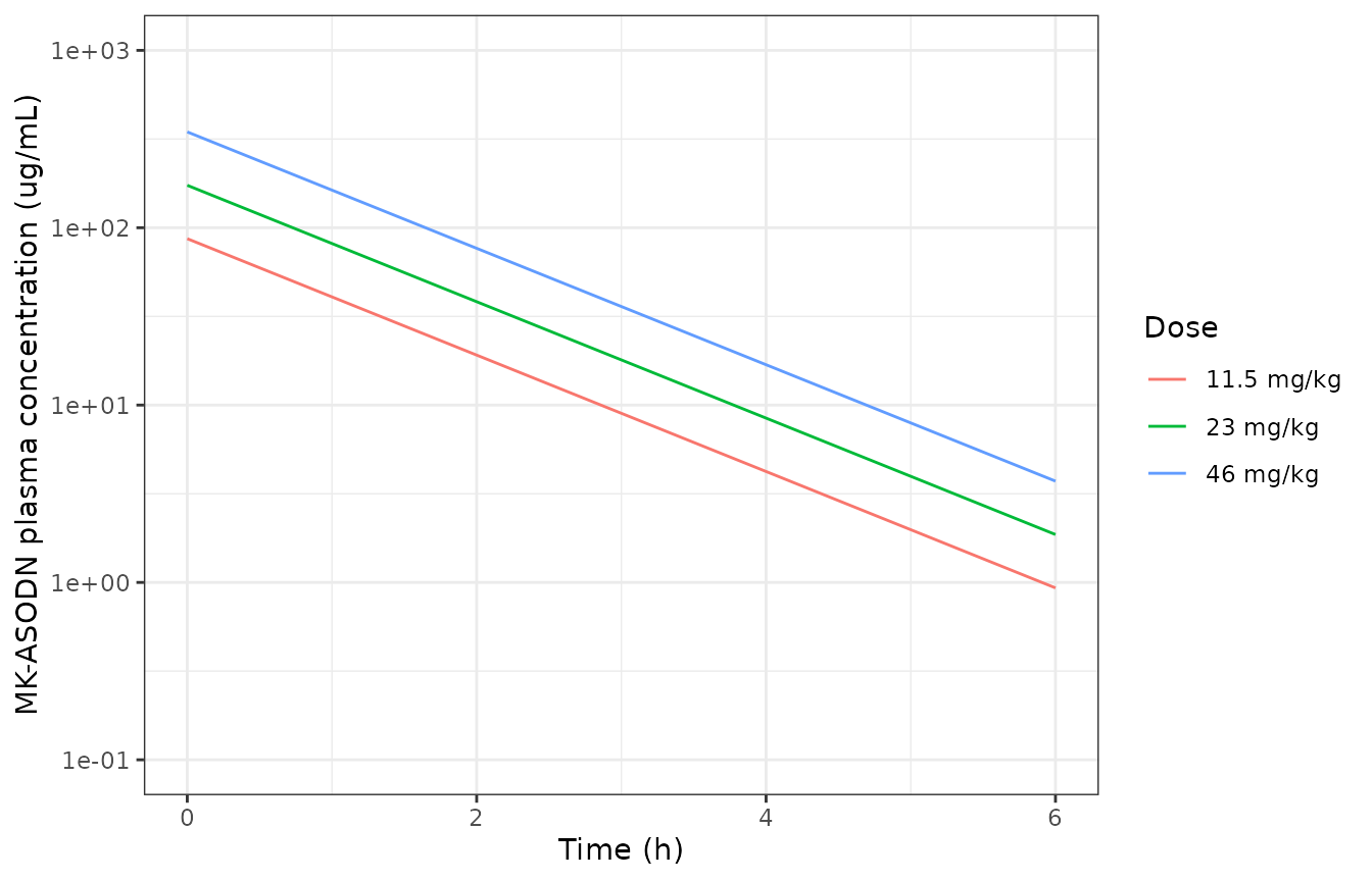
Replicates the simulated (solid-line) curves of Figure 1 of Bai 2021: monkey plasma concentration after a single IV injection of 11.5, 23 and 46 mg/kg. The reduction omits the sub-10-minute initial spike that the whole-body model draws at t = 0.
sim_human |>
  dplyr::filter(time <= 6) |>
  ggplot(aes(time, Cc)) +
  geom_line(colour = "blue") +
  scale_y_log10(limits = c(0.1, 100)) +
  labs(x = "Time (h)", y = "MK-ASODN plasma concentration (ug/mL)") +
  theme_bw()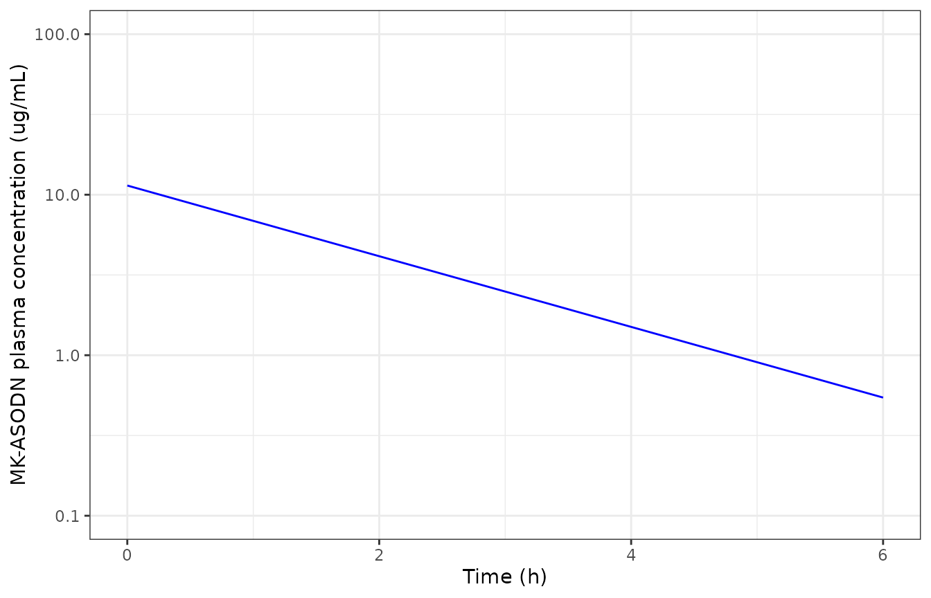
Replicates Figure 3 of Bai 2021: predicted human plasma concentration after a single 90 mg IV injection.
PKNCA validation
sim_all <- dplyr::bind_rows(sim_monkey, sim_human)

sim_nca <- sim_all |>
  dplyr::filter(!is.na(Cc)) |>
  dplyr::select(id, time, Cc, treatment)

# Guarantee a time = 0 row per subject (IV bolus; rxode2 returns the post-dose
# concentration at t = 0, which is kept by distinct()).
sim_nca <- dplyr::bind_rows(
  sim_nca,
  sim_nca |> dplyr::distinct(id, treatment) |> dplyr::mutate(time = 0, Cc = 0)
) |>
  dplyr::distinct(id, time, .keep_all = TRUE) |>
  dplyr::arrange(id, time)

conc_obj <- PKNCA::PKNCAconc(sim_nca, Cc ~ time | treatment + id,
                             concu = "mg/L", timeu = "h")

dose_df <- dplyr::bind_rows(ev_monkey, ev_human) |>
  dplyr::filter(evid == 1) |>
  dplyr::select(id, time, amt, treatment)

dose_obj <- PKNCA::PKNCAdose(dose_df, amt ~ time | treatment + id,
                             doseu = "mg")

intervals <- data.frame(
  start = 0, end = Inf,
  cmax = TRUE, aucinf.obs = TRUE, half.life = TRUE
)

nca_res <- PKNCA::pk.nca(PKNCA::PKNCAdata(conc_obj, dose_obj,
                                          intervals = intervals))
#> Warning: treatment=Human 90 mg; id=10: No concentration data
Comparison against the paper’s own PBPK predictions
The reduction’s job is to reproduce what the whole-body model predicted, so Table 4’s predicted values are the reference.
published <- tibble::tribble(
  ~treatment,     ~cmax,  ~aucinf.obs,
  "11.5 mg/kg",   84.09,       114.77,
  "23 mg/kg",    172.00,       229.54,
  "46 mg/kg",    341.00,       459.09,
  "Human 90 mg",  49.98,        22.48
)

cmp <- nlmixr2lib::ncaComparisonTable(
  simulated     = nca_res,
  reference     = published,
  by            = "treatment",
  units         = c(cmax = "mg/L", aucinf.obs = "mg*h/L"),
  tolerance_pct = 20
)

knitr::kable(
  cmp,
  caption = paste(
    "Reduced models vs the GastroPlus PBPK predictions in Table 4 of Bai 2021.",
    "* marks a difference above 20%. The only starred row is the human Cmax,",
    "which is the platform's instantaneous-bolus spike; see Assumptions and",
    "deviations."
  )
)| NCA parameter | treatment | Reference | Simulated | % diff |
|---|---|---|---|---|
| Cmax (mg/L) | 11.5 mg/kg | 84.1 | 86.7 | +3.1% |
| Cmax (mg/L) | 23 mg/kg | 172 | 173 | +0.8% |
| Cmax (mg/L) | 46 mg/kg | 341 | 347 | +1.7% |
| Cmax (mg/L) | Human 90 mg | 50 | 11.4 | -77.2%* |
| AUC0-∞ (obs) (mg*h/L) | 11.5 mg/kg | 115 | 115 | +0.0% |
| AUC0-∞ (obs) (mg*h/L) | 23 mg/kg | 230 | 230 | +0.0% |
| AUC0-∞ (obs) (mg*h/L) | 46 mg/kg | 459 | 459 | -0.0% |
| AUC0-∞ (obs) (mg*h/L) | Human 90 mg | 22.5 | 22.5 | +0.1% |
sim_wide <- as.data.frame(nca_res) |>
  dplyr::select(treatment, PPTESTCD, PPORRES) |>
  tidyr::pivot_wider(names_from = PPTESTCD, values_from = PPORRES)

score <- published |>
  dplyr::left_join(sim_wide, by = "treatment", suffix = c("_pub", "_sim")) |>
  dplyr::mutate(
    auc_ratio  = aucinf.obs_sim / aucinf.obs_pub,
    cmax_ratio = cmax_sim / cmax_pub
  )

# The join must have matched every published row.
stopifnot(nrow(score) == 4, !anyNA(score$auc_ratio), !anyNA(score$cmax_ratio))

score |>
  dplyr::select(treatment, aucinf.obs_pub, aucinf.obs_sim, auc_ratio,
                cmax_pub, cmax_sim, cmax_ratio, half.life) |>
  dplyr::rename(
    "Scenario" = treatment,
    "AUC published" = aucinf.obs_pub, "AUC simulated" = aucinf.obs_sim,
    "AUC ratio" = auc_ratio,
    "Cmax published" = cmax_pub, "Cmax simulated" = cmax_sim,
    "Cmax ratio" = cmax_ratio, "t1/2 simulated (h)" = half.life
  ) |>
  knitr::kable(digits = 3,
caption = "Reduced model / published PBPK prediction, per scenario.")| Scenario | AUC published | AUC simulated | AUC ratio | Cmax published | Cmax simulated | Cmax ratio | t1/2 simulated (h) |
|---|---|---|---|---|---|---|---|
| 11.5 mg/kg | 114.77 | 114.771 | 1.000 | 84.09 | 86.727 | 1.031 | 0.917 |
| 23 mg/kg | 229.54 | 229.541 | 1.000 | 172.00 | 173.454 | 1.008 | 0.917 |
| 46 mg/kg | 459.09 | 459.082 | 1.000 | 341.00 | 346.908 | 1.017 | 0.917 |
| Human 90 mg | 22.48 | 22.500 | 1.001 | 49.98 | 11.407 | 0.228 | 1.367 |
# Deterministic comparisons, so tight bounds are correct.
# AUC reproduces the PBPK prediction on every scenario.
stopifnot(max(abs(score$auc_ratio - 1)) < 0.01)

# Monkey Cmax reproduces the tabulated prediction (start of the terminal
# phase) on all three arms.
monkey <- score |> dplyr::filter(treatment != "Human 90 mg")
stopifnot(max(abs(monkey$cmax_ratio - 1)) < 0.05)

# Human Cmax: the reduction starts at dose / Vss = 11.4 ug/mL, i.e. about
# 0.23 of the platform's bolus spike. Pinned so a change in structure or
# volume shows up here.
human <- score |> dplyr::filter(treatment == "Human 90 mg")
stopifnot(abs(human$cmax_sim - 90 / 7.89) < 0.01,
          abs(human$cmax_ratio - 0.228) < 0.005)

# Half-lives: monkey 0.917 h from the digitised Figure 1 slope, human
# ln2 * 7.89 / 4 = 1.367 h.
stopifnot(max(abs(monkey$half.life / (log(2) * 0.1326 / 0.1002) - 1)) < 0.01,
          abs(human$half.life / t12_identity - 1) < 0.01)
Comparison against the observed monkey data
The monkey NCA in Table 1 is observed data, which the whole-body model itself fits only approximately. The paper’s own fold errors are 2.22, 2.00 and 1.73 on Cmax and 0.94, 0.98 and 1.10 on AUC (Table 4). The reduction inherits those, because its AUC equals the PBPK prediction.
observed <- tibble::tribble(
  ~treatment,    ~auc_obs, ~cmax_obs, ~t12_obs, ~cl_obs_mlkgh, ~vss_obs_mlkg,
  "11.5 mg/kg",    122.04,    187.16,     0.79,         95.41,         88.41,
  "23 mg/kg",      232.87,    347.43,     1.08,         99.16,        104.63,
  "46 mg/kg",      415.38,    588.73,     1.33,        110.95,        137.89
)

obs_cmp <- observed |>
  dplyr::left_join(sim_wide, by = "treatment") |>
  dplyr::mutate(auc_sim_over_obs = aucinf.obs / auc_obs,
                cmax_sim_over_obs = cmax / cmax_obs)
stopifnot(nrow(obs_cmp) == 3, !anyNA(obs_cmp$auc_sim_over_obs))

obs_cmp |>
  dplyr::select(treatment, auc_obs, aucinf.obs, auc_sim_over_obs,
                cmax_obs, cmax, cmax_sim_over_obs, t12_obs, half.life) |>
  dplyr::rename(
    "Dose" = treatment,
    "AUC observed" = auc_obs, "AUC simulated" = aucinf.obs,
    "AUC sim/obs" = auc_sim_over_obs,
    "Cmax observed" = cmax_obs, "Cmax simulated" = cmax,
    "Cmax sim/obs" = cmax_sim_over_obs,
    "t1/2 observed (h)" = t12_obs, "t1/2 simulated (h)" = half.life
  ) |>
  knitr::kable(digits = 3,
caption = "Reduced monkey model vs observed monkey NCA (Table 1 of Bai 2021).")| Dose | AUC observed | AUC simulated | AUC sim/obs | Cmax observed | Cmax simulated | Cmax sim/obs | t1/2 observed (h) | t1/2 simulated (h) |
|---|---|---|---|---|---|---|---|---|
| 11.5 mg/kg | 122.04 | 114.771 | 0.940 | 187.16 | 86.727 | 0.463 | 0.79 | 0.917 |
| 23 mg/kg | 232.87 | 229.541 | 0.986 | 347.43 | 173.454 | 0.499 | 1.08 | 0.917 |
| 46 mg/kg | 415.38 | 459.082 | 1.105 | 588.73 | 346.908 | 0.589 | 1.33 | 0.917 |
# The paper's own AUC fold errors (0.94-1.10) carried over.
stopifnot(all(obs_cmp$auc_sim_over_obs > 0.9 & obs_cmp$auc_sim_over_obs < 1.15))
The observed monkey data are less than dose-proportional (the observed clearance rises from 95 to 111 mL/h/kg and the half-life from 0.79 to 1.33 h across the dose range; Table 2 calls dose proportionality “inconclusive”). The PBPK model, and therefore both reductions, is linear and does not reproduce that trend.
Assumptions and deviations
- The whole-body structure is not reproduced. The 14-tissue GastroPlus model uses the software’s default monkey and human physiology and Rodgers-Single Kp values, none of which is printed. Both files encode the plasma-level behaviour the paper’s own outputs pin down, not the platform model.
- Monkey clearance is back-solved, not printed. Methods 2.7 says the monkey PBPK used the in vivo clearance but does not say which value. Dose / predicted AUC0-inf gives 0.10020 L/h/kg on all three arms. That is close to, but not equal to, the mean of the three observed NCA clearances (101.8 mL/h/kg, Table 1).
- Monkey volume is digitised. No monkey model volume is printed. The maintainers digitised the simulated curves of Figure 1 by pixel regression over the terminal phase (1.7-5.9 h). Panels A and B give V = CL / k = 0.1326 L/kg to four digits. Panel C, on a coarser axis, gives 0.1341. The reduced model then reproduces Table 4’s predicted AUC (by construction) and predicted Cmax (independently, within 3.1%).
- Monkey per-kg scaling is linear, referenced to 6 kg. The paper reports clearance per kg and doses per kg, so clearance and volume scale with body weight to the power 1. The 6 kg reference is the approximate weight stated in Methods 2.2. Under mg/kg dosing, concentrations do not depend on the weight chosen.
-
The initial spike is not carried. Both GastroPlus
curves (Figures 1 and
- start with a sub-10-minute spike, from the bolus mixing into a small plasma volume before tissue distribution. It holds under 2% of the AUC. The human Table 4 Cmax (49.98 ug/mL) is that spike, so the reduction gives 11.4 ug/mL (ratio 0.23). The monkey Table 4 Cmax values are not the spike (they equal dose / V at the start of the terminal phase), so the reduction reproduces them. A two-compartment fit to the spike would need values the paper does not print. The bolus Cmax is therefore a known limitation of the human file: do not use it to predict a peak concentration within the first few minutes after an injection.
- The human prediction is a single virtual subject. The paper prints human CL and Vss but neither body weight in its allometric equation CL_human = CL_monkey x (BW_human / BW_monkey)^0.8. With the monkey clearance above (0.6012 L/h at 6 kg), CL_human = 4 L/h implies a human weight of about 64 kg. That is arithmetic, not a printed value, so the human file carries no weight covariate.
-
No variability. The paper reports no
interindividual or residual variability for either simulation. No etas
are declared, and
addSd/propSdarefixed(0). - Protein binding. Human plasma protein binding was 96-99% (Table 3). The paper reports only total concentrations, so no unbound concentration is computed.
- Errata. No erratum or correction for this article was found in a check of Europe PMC (PMID 34803711; no linked correction, and no erratum matching the article) on 2026-09-29.