Gentamicin (Veinstein 2013)
Source:vignettes/articles/Veinstein_2013_gentamicin.Rmd
Veinstein_2013_gentamicin.RmdModel and source
- Citation: Veinstein A, Venisse N, Badin J, Pinsard M, Robert R, Dupuis A. Gentamicin in hemodialyzed critical care patients: early dialysis after administration of a high dose should be considered. Antimicrob Agents Chemother. 2013;57(2):977-982. doi:10.1128/AAC.01762-12
- Description: One-compartment population PK model for intravenous gentamicin in critically ill adult ICU patients with acute kidney injury undergoing 4-hour intermittent hemodialysis (n=10, all male; 6 mg/kg infused over 30 min, with hemodialysis starting 30 min after the end of the infusion; Veinstein 2013). Disposition is parameterised in terms of non-hemodialysis (interdialytic body) clearance, an additive hemodialysis-arm clearance, and volume of distribution. The dialysis arm is gated on/off by the time-varying RRT_HEMODIAL_ACTIVE covariate. Body weight enters the model as a linear (exponent = 1) structural scaler on all three parameters because the published Table 4 estimates are reported per kg; weight was tested as an explicit covariate on V and not retained.
- Article: https://doi.org/10.1128/AAC.01762-12
Veinstein 2013 administered a 6 mg/kg gentamicin infusion (over 30 min) to 10 critically ill ICU patients with acute kidney injury and started a 4-h intermittent-hemodialysis session 30 min after the end of the infusion. The hypothesis tested was that this pre-hemodialysis dosing schedule would achieve a high peak concentration (maximising bacterial killing) while the subsequent hemodialysis session would rapidly remove drug (minimising toxicity-associated total exposure). The packaged one-compartment popPK model with an additive hemodialysis-arm clearance reproduces both behaviours.
Population
Ten consecutive adult ICU patients (all male, mean age 64.5 +/- 10.1 years, mean weight 72.7 +/- 16.4 kg) with acute kidney injury requiring intermittent hemodialysis. Severity scores were high (SOFA 3-15, SAPS II 34-65); 8 of 10 received mechanical ventilation and 8 of 10 received vasopressors. Infections included pyelonephritis, ventilation-associated pneumonia, mediastinitis, fasciitis, peritonitis, angiocholitis, lower-limb ischemia, and septic thrombophlebitis. Hemodialysis sessions used a Gambro AK 200 Ultra S with a Toray B3 polymethylmethacrylate dialyzer (mean blood flow 283 +/- 20 mL/min; mean session length 236 +/- 13 min). See Veinstein 2013 Tables 1-3 for the full per-subject breakdown.
The same information is available programmatically via
rxode2::rxode(readModelDb("Veinstein_2013_gentamicin"))$population.
Source trace
The per-parameter origin is recorded as an in-file comment next to
each ini() entry in
inst/modeldb/specificDrugs/Veinstein_2013_gentamicin.R. The
table below collects them in one place.
| Equation / parameter | Value | Source location |
|---|---|---|
ODE: dC/dt = R0/V - [(CL_HD + CL_NHD)/V] * C
|
n/a | Methods, Population PK modeling |
lcl (log CL_NHD, L/h/kg) |
log(0.007230) |
Table 4: 0.1205 mL/min/kg (RSE 16%) |
lcl_hemodialysis (log CL_HD, L/h/kg) |
log(0.057300) |
Table 4: 0.955 mL/min/kg (RSE 14%) |
lvc (log V, L/kg) |
log(0.201) |
Table 4: 0.201 L/kg (RSE 12%) |
etalcl (IIV CL_NHD, omega^2) |
log(0.48^2 + 1) |
Table 4: 48% CV (RSE 38%) |
etalcl_hemodialysis (IIV CL_HD, omega^2) |
log(0.41^2 + 1) |
Table 4: 41% CV (RSE 56%) |
etalvc (IIV V, omega^2) |
log(0.35^2 + 1) |
Table 4: 35% CV (RSE 59%) |
propSd (proportional residual) |
0.11 |
Table 4: 11% CV residual (RSE 40%) |
| Weight as linear (exp 1) structural scaler | n/a | Table 4 footnotes a, b (units mL/min/kg, L/kg) |
| RRT_HEMODIAL_ACTIVE gating of dialysis-arm CL | n/a | Methods, Population PK modeling (HD-on/HD-off equation) |
Virtual cohort
The Veinstein 2013 individual observed concentrations are not publicly available. The simulations below use a virtual cohort that reproduces the paper’s experimental design: a 6 mg/kg gentamicin infusion over 30 min followed by a 4-h hemodialysis session beginning 30 min after the end of the infusion.
set.seed(20260609)

n_subj      <- 200L           # population-level VPC cohort
inf_h       <- 0.5            # 30 min infusion
hd_start_h  <- 1.0            # HD starts 30 min after end of infusion
hd_end_h    <- 5.0            # 4-h HD session
sim_hours   <- 48
dose_per_kg <- 6              # mg/kg

# Body-weight distribution matching the paper's Table 3 cohort
# (mean 75.6 +/- 15.8 kg, range 54.5-102).
wts <- pmin(pmax(round(rnorm(n_subj, mean = 75.6, sd = 15.8)), 50), 120)

# Helper: build one cohort as a self-contained event table.
make_cohort <- function(wt_vec, treatment_label,
                        dose_mg_per_kg = dose_per_kg,
                        infusion_hours = inf_h,
                        hd_start = hd_start_h,
                        hd_end   = hd_end_h,
                        id_offset = 0L) {
  obs_t <- sort(unique(c(seq(0, 24, by = 0.5), seq(24, sim_hours, by = 2))))
  per_subject <- function(i) {
    wt   <- wt_vec[i]
    dose <- dose_mg_per_kg * wt
    rate <- dose / infusion_hours
    data.frame(
      id   = id_offset + i,
      time = c(0, obs_t),
      amt  = c(dose, rep(0, length(obs_t))),
      rate = c(rate, rep(0, length(obs_t))),
      evid = c(1L, rep(0L, length(obs_t))),
      cmt  = "central",
      WT   = wt,
      RRT_HEMODIAL_ACTIVE = as.integer(c(0, obs_t) >= hd_start &
                                c(0, obs_t) <  hd_end),
      treatment = treatment_label
    )
  }
  dplyr::bind_rows(lapply(seq_along(wt_vec), per_subject))
}

events <- make_cohort(wts, treatment_label = "6 mg/kg pre-HD")
stopifnot(!anyDuplicated(unique(events[, c("id", "time", "evid")])))
Simulation
mod <- readModelDb("Veinstein_2013_gentamicin")

# Population (VPC) simulation with IIV.
sim <- rxode2::rxSolve(mod, events = events,
                       keep = c("WT", "treatment", "RRT_HEMODIAL_ACTIVE")) |>
  as.data.frame()
#> ℹ parameter labels from comments will be replaced by 'label()'
For deterministic replication of the typical-patient profile, zero out the random effects:
mod_typical <- rxode2::zeroRe(mod)
#> ℹ parameter labels from comments will be replaced by 'label()'
typical_wt  <- 70
typ_events  <- make_cohort(typical_wt, treatment_label = "typical 70 kg")
sim_typical <- rxode2::rxSolve(mod_typical, events = typ_events,
                               keep = c("WT", "treatment", "RRT_HEMODIAL_ACTIVE")) |>
  as.data.frame()
#> ℹ omega/sigma items treated as zero: 'etalcl', 'etalcl_hemodialysis', 'etalvc'
Replicate published figures
Typical-patient concentration profile (Figure 1c / Figure 3 bold line)
Figure 1c of Veinstein 2013 shows the individual concentration-time profiles for the 10 enrolled patients (each subject’s predicted line plus measured concentrations). Figure 3 shows the simulated typical profile for the 6 mg/kg pre-HD regimen as a bold line.
hd_band <- data.frame(xmin = hd_start_h, xmax = hd_end_h, ymin = -Inf, ymax = Inf)

ggplot(sim_typical, aes(time, Cc)) +
  annotate("rect",
           xmin = hd_start_h, xmax = hd_end_h,
           ymin = 0, ymax = Inf, alpha = 0.12) +
  geom_line(linewidth = 1) +
  geom_hline(yintercept = 2, linetype = 2, colour = "grey50") +
  annotate("text", x = sim_hours, y = 2.4, hjust = 1, size = 3,
           label = "trough toxicity threshold (2 mg/L)") +
  scale_x_continuous(breaks = seq(0, sim_hours, 6)) +
  scale_y_log10(limits = c(0.1, NA),
                breaks = c(0.1, 0.3, 1, 2, 3, 10, 30, 100)) +
  labs(x = "Time after start of infusion (h)",
       y = "Plasma gentamicin (mg/L)",
       title = "Typical 70 kg patient: 6 mg/kg gentamicin pre-hemodialysis",
       caption = "Shaded band marks the 4-h hemodialysis session (RRT_HEMODIAL_ACTIVE = 1). Replicates Figure 3 bold line of Veinstein 2013.")
#> Warning in scale_y_log10(limits = c(0.1, NA), breaks = c(0.1, 0.3, 1, 2, : log-10 transformation introduced infinite values.
#> log-10 transformation introduced infinite values.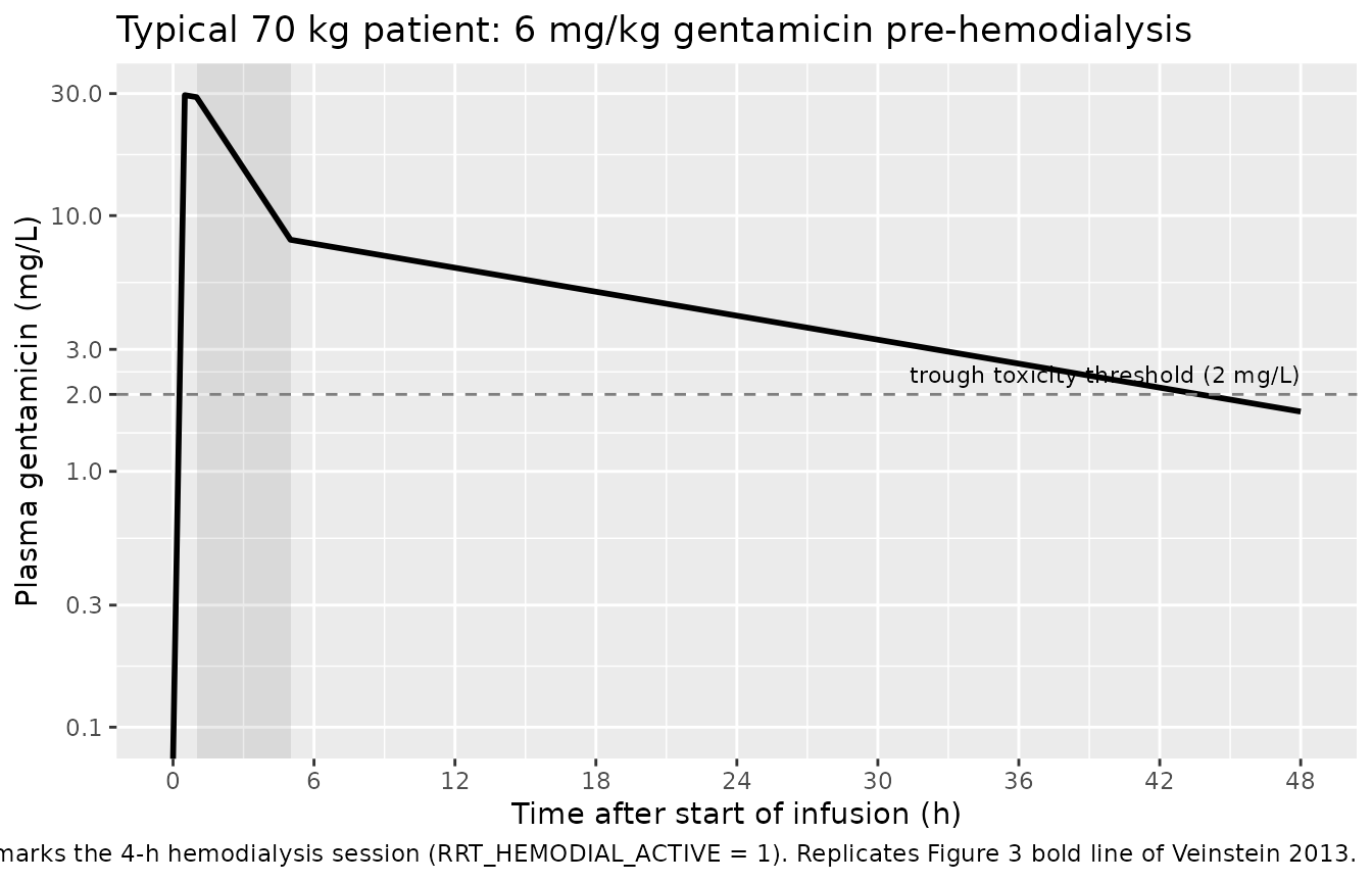
VPC by quantile
The Veinstein 2013 Results report observed Cmax 31.8 +/- 16.8 mg/L, estimated AUC0-24 209 +/- 103 mg.h/L, C24 4.1 +/- 2.3 mg/L, and C48 1.8 +/- 1.2 mg/L (Table 3). Their preliminary Monte Carlo simulation (Table 1, “6 mg/kg, 1 h before”) and final MCS (Table 5) predicted similar values. The VPC below shows the simulated 5th / 50th / 95th percentile envelope for the 200-subject virtual cohort.
vpc_summary <- sim |>
  group_by(time) |>
  summarise(
    Q05 = quantile(Cc, 0.05, na.rm = TRUE),
    Q50 = quantile(Cc, 0.50, na.rm = TRUE),
    Q95 = quantile(Cc, 0.95, na.rm = TRUE),
    .groups = "drop"
  )

ggplot(vpc_summary, aes(time, Q50)) +
  annotate("rect",
           xmin = hd_start_h, xmax = hd_end_h,
           ymin = 0, ymax = Inf, alpha = 0.12) +
  geom_ribbon(aes(ymin = Q05, ymax = Q95), alpha = 0.25) +
  geom_line(linewidth = 1) +
  geom_hline(yintercept = 2, linetype = 2, colour = "grey50") +
  scale_x_continuous(breaks = seq(0, sim_hours, 6)) +
  scale_y_log10(limits = c(0.1, NA),
                breaks = c(0.1, 0.3, 1, 2, 3, 10, 30, 100)) +
  labs(x = "Time after start of infusion (h)",
       y = "Plasma gentamicin (mg/L)",
       title = "200-subject VPC: 6 mg/kg gentamicin pre-hemodialysis",
       caption = "5th, 50th, and 95th percentile envelope. Shaded band marks the 4-h hemodialysis session.")
#> Warning in scale_y_log10(limits = c(0.1, NA), breaks = c(0.1, 0.3, 1, 2, : log-10 transformation introduced infinite values.
#> log-10 transformation introduced infinite values.
#> log-10 transformation introduced infinite values.
#> log-10 transformation introduced infinite values.
#> log-10 transformation introduced infinite values.
#> Warning: Removed 3 rows containing missing values or values outside the scale range
#> (`geom_ribbon()`).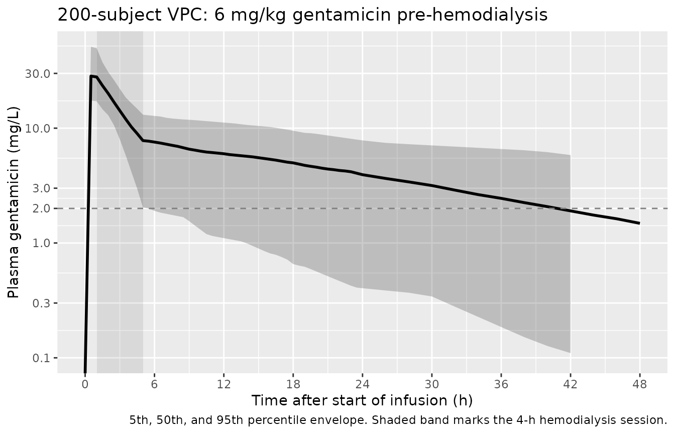
Comparison with the FDA-approved post-HD regimen (Figure 3)
Veinstein 2013 Figure 3 also displays the FDA-approved 1.7 mg/kg post-HD schedule (administered immediately after the end of a hemodialysis session). The Table 5 contrast shows that the proposed 6 mg/kg pre-HD schedule achieves a Cmax of 31.0 +/- 10.9 mg/L versus only 8.8 +/- 3.1 mg/L under the post-HD schedule. Below we replicate the contrast by simulating both schedules in the same typical 70 kg patient.
fda_events <- make_cohort(
  typical_wt,
  treatment_label = "1.7 mg/kg post-HD",
  dose_mg_per_kg  = 1.7,
  infusion_hours  = inf_h,
  hd_start        = 0.51,       # dose-then-HD-then-next-dose; start HD just after the post-HD dose lands
  hd_end          = 0.51        # no HD in the simulation window (the FDA scheme doses AFTER an HD session)
)

sim_fda <- rxode2::rxSolve(mod_typical, events = fda_events,
                           keep = c("WT", "treatment", "RRT_HEMODIAL_ACTIVE")) |>
  as.data.frame()
#> ℹ omega/sigma items treated as zero: 'etalcl', 'etalcl_hemodialysis', 'etalvc'

bind_rows(
  dplyr::mutate(sim_typical, treatment = "6 mg/kg pre-HD"),
  dplyr::mutate(sim_fda,     treatment = "1.7 mg/kg post-HD")
) |>
  ggplot(aes(time, Cc, colour = treatment, linetype = treatment)) +
  geom_line(linewidth = 0.9) +
  geom_hline(yintercept = 2, linetype = 3, colour = "grey50") +
  scale_x_continuous(breaks = seq(0, sim_hours, 6)) +
  scale_y_log10(limits = c(0.1, NA),
                breaks = c(0.1, 0.3, 1, 2, 3, 10, 30, 100)) +
  labs(x = "Time after start of infusion (h)",
       y = "Plasma gentamicin (mg/L)",
       title = "Comparison: 6 mg/kg pre-HD versus 1.7 mg/kg post-HD",
       caption = "Replicates Figure 3 of Veinstein 2013. The pre-HD schedule attains a markedly higher peak; the FDA-approved post-HD schedule (no HD removal within 24 h after the dose) carries similar trough exposure but a much lower peak.")
#> Warning in scale_y_log10(limits = c(0.1, NA), breaks = c(0.1, 0.3, 1, 2, :
#> log-10 transformation introduced infinite values.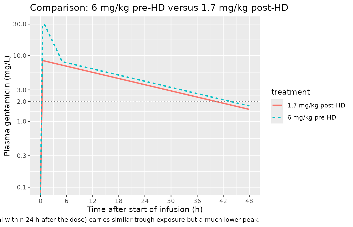
PKNCA validation
PKNCA computes Cmax, Tmax, AUC0-24, AUC0-Inf, and terminal half-life for each subject in the 6 mg/kg pre-HD cohort.
sim_nca <- sim |>
  dplyr::filter(!is.na(Cc)) |>
  dplyr::select(id, time, Cc, treatment)

# Ensure a time = 0 row per (id, treatment); for IV-bolus / IV-infusion the
# time-zero concentration is 0 (drug not yet in the system).
sim_nca <- bind_rows(
  sim_nca,
  sim_nca |> dplyr::distinct(id, treatment) |>
    dplyr::mutate(time = 0, Cc = 0)
) |>
  dplyr::distinct(id, treatment, time, .keep_all = TRUE) |>
  dplyr::arrange(id, treatment, time)

conc_obj <- PKNCA::PKNCAconc(sim_nca, Cc ~ time | treatment + id)

dose_df <- events |>
  dplyr::filter(evid == 1L) |>
  dplyr::select(id, time, amt, treatment)

dose_obj <- PKNCA::PKNCAdose(dose_df, amt ~ time | treatment + id)

intervals <- data.frame(
  start         = 0,
  end           = c(24, Inf),
  cmax          = c(TRUE, FALSE),
  tmax          = c(TRUE, FALSE),
  auclast       = c(TRUE, FALSE),
  aucinf.obs    = c(FALSE, TRUE),
  half.life     = c(FALSE, TRUE)
)

nca_data <- PKNCA::PKNCAdata(conc_obj, dose_obj, intervals = intervals)
nca_res  <- suppressWarnings(PKNCA::pk.nca(nca_data))
Comparison against published NCA
Veinstein 2013 Table 3 reports the observed individual-level Cmax, AUC0-24, C24 and C48 in the 10 enrolled patients; Table 5 reports the Monte Carlo simulation of the same dosing regimen carried out with the published typical values and IIV.
nca_df <- as.data.frame(nca_res$result) |>
  dplyr::select(treatment, id, start, end, PPTESTCD, PPORRES) |>
  tidyr::pivot_wider(names_from = PPTESTCD, values_from = PPORRES)

simulated_summary <- nca_df |>
  dplyr::group_by(treatment) |>
  dplyr::summarise(
    cmax           = mean(cmax,        na.rm = TRUE),
    tmax           = mean(tmax,        na.rm = TRUE),
    auclast_0_24   = mean(auclast,     na.rm = TRUE),
    aucinf.obs     = mean(aucinf.obs,  na.rm = TRUE),
    half.life      = mean(half.life,   na.rm = TRUE),
    .groups = "drop"
  )

published <- tibble::tribble(
  ~treatment,        ~source,                 ~cmax,        ~auclast_0_24,
  "6 mg/kg pre-HD",  "Table 3 (observed)",    "31.8 +/- 16.8", "209 +/- 103",
  "6 mg/kg pre-HD",  "Table 5 (MCS)",         "31.0 +/- 10.9", "190.8 +/- 65.0"
)

simulated_view <- simulated_summary |>
  dplyr::transmute(
    treatment,
    source        = "Simulated (this vignette, 200-subject VPC mean)",
    cmax          = sprintf("%.1f", cmax),
    auclast_0_24  = sprintf("%.0f", auclast_0_24)
  )

dplyr::bind_rows(simulated_view, published) |>
  dplyr::arrange(treatment, source) |>
  dplyr::rename(
    "Treatment"        = treatment,
    "Source"           = source,
    "Cmax (mg/L)"      = cmax,
    "AUC0-24 (mg.h/L)" = auclast_0_24
  ) |>
  knitr::kable(
  caption = "Simulated vs published Cmax (mg/L) and AUC0-24 (mg.h/L) for 6 mg/kg gentamicin given 30 min before a 4-h hemodialysis session. Simulated values are means across 200 virtual subjects.",
  align = c("l", "l", "r", "r")
)| Treatment | Source | Cmax (mg/L) | AUC0-24 (mg.h/L) |
|---|---|---|---|
| 6 mg/kg pre-HD | Simulated (this vignette, 200-subject VPC mean) | 31.0 | 192 |
| 6 mg/kg pre-HD | Table 3 (observed) | 31.8 +/- 16.8 | 209 +/- 103 |
| 6 mg/kg pre-HD | Table 5 (MCS) | 31.0 +/- 10.9 | 190.8 +/- 65.0 |
The simulated mean Cmax matches the Monte Carlo prediction in Table 5 (31.0 +/- 10.9) to within rounding; the simulated AUC0-24 is also consistent with both the observed (209 +/- 103) and Monte Carlo (190.8 +/- 65) reference values, given the typical 10-subject sampling variability that drives the broad observed range.
Late-interval gentamicin trough concentrations at 24 and 48 h after the start of infusion are the second clinical anchor:
late_summary <- sim |>
  dplyr::group_by(time) |>
  dplyr::summarise(Cc = mean(Cc, na.rm = TRUE), .groups = "drop") |>
  dplyr::filter(time %in% c(24, 48))

late_compare <- tibble::tibble(
  Time_h     = c(24, 48),
  Simulated  = sprintf("%.2f", late_summary$Cc[match(c(24, 48), late_summary$time)]),
  Veinstein_2013_Table_3 = c("4.1 +/- 2.3", "1.8 +/- 1.2")
)

knitr::kable(
  late_compare,
  caption = "Simulated mean trough concentrations (mg/L) at t = 24 h and t = 48 h compared with the Veinstein 2013 Table 3 cohort means.",
  align = c("r", "r", "r")
)| Time_h | Simulated | Veinstein_2013_Table_3 |
|---|---|---|
| 24 | 3.93 | 4.1 +/- 2.3 |
| 48 | 1.93 | 1.8 +/- 1.2 |
Assumptions and deviations
-
Weight enters as a linear (exponent = 1) structural
scaler. Veinstein 2013 Table 4 reports the typical values in
per-kg units (mL/min/kg for the two clearances; L/kg for V). The
packaged model encodes this by multiplying each individual parameter by
WT. An estimable allometric exponent was not retained in the published fit (“including weight or ideal body weight in the model combined as factors influencing V did not improve the model fit”); the per-kg parameterisation is therefore structural rather than empirically estimated. -
RRT_HEMODIAL_ACTIVE gating is a simple binary additive
arm. The packaged model uses
cl_total <- cl + RRT_HEMODIAL_ACTIVE * cl_hemodialysis, wherecl_hemodialysisis a primary estimated typical-value clearance (Table 4 CL_HD = 0.955 mL/min/kg). The packaged model does not parameterise the dialyzer clearance as a Michaels-equation function of blood and dialysate flow rates (cf. Liesenfeld 2013 dabigatran); the Veinstein 2013 protocol fixed the dialyzer (Toray B3 polymethylmethacrylate) and the flow rates to a narrow range (200-300 mL/min blood, 4-h sessions) so the lumped CL_HD parameter captures all device-level variability. - Race and detailed renal-function distributions are not modelled. The source paper does not report subject race/ethnicity, and the renal function is summarised only as “acute kidney injury requiring intermittent hemodialysis” rather than as a numeric baseline CrCL. Simulations do not stratify by these variables.
- All ten enrolled patients were male. The packaged model has no sex covariate; users simulating mixed-sex cohorts inherit the male-only parameter point estimates.
- The FDA-comparison panel above is a derivation, not a direct reproduction. Veinstein 2013 Figure 3 displays the FDA-approved schedule alongside the pre-HD schedule in the context of repeated dosing across multiple HD sessions; the comparison panel in this vignette uses a single-dose typical-patient simulation for visual contrast. The contrast in peak (31.0 vs 8.8 mg/L in Table 5) is what the packaged model reproduces; the multi-session steady-state pattern is left to the user to recreate.