Alirocumab LDL-C indirect response (Nicolas 2019)

Model and source

Citation: Nicolas X, Djebli N, Rauch C, Brunet A, Hurbin F, Martinez JM, Fabre D. Population Pharmacokinetic/Pharmacodynamic Analysis of Alirocumab in Healthy Volunteers or Hypercholesterolemic Subjects Using an Indirect Response Model to Predict Low-Density Lipoprotein Cholesterol Lowering: Support for a Biologics License Application Submission: Part II. Clin Pharmacokinet. 2019;58(1):115-130. doi:10.1007/s40262-018-0670-5
Description: Sequential population PK/PD model for alirocumab and serum LDL cholesterol in healthy volunteers and adults with hypercholesterolemia (Nicolas 2019, Part II). A type IV (stimulation-of-loss) indirect response model with a Hill coefficient links total alirocumab concentration to LDL-C elimination; the PK layer is the Michaelis-Menten target-mediated approximation of Martinez 2019 (Part I), carried fixed as the concentration driver. Ten covariates act on the four PD parameters (Emax, EC50, Hill coefficient and Kout).
Article: https://doi.org/10.1007/s40262-018-0670-5
Electronic supplementary material (open access): https://doi.org/10.1007/s40262-018-0670-5 (ESM Tables 1-3, ESM Figures 1-3)
Companion Part I population PK paper: https://doi.org/10.1007/s40262-018-0669-y, packaged as Martinez_2019_alirocumab

Nicolas 2019 is Part II of a two-part Biologics License Application support package. Part I (Martinez 2019) developed the alirocumab population PK model; Part II fixes that PK and fits an LDL-cholesterol indirect response model to the predicted concentrations. The model packaged here is the combination: the Part I PK structure carried fixed as the concentration driver, plus the Part II PD layer. Nothing in the PK layer was re-estimated by Nicolas 2019, and every PK ini() entry is wrapped in fixed() to record that.

Population

The analysis pooled 2799 individuals contributing 14,346 LDL-C values across 13 phase I/II/III trials (Nicolas 2019 Table 1). The cohort was 2649 (94.6%) patients with heterozygous familial or non-familial hypercholesterolemia – several with established coronary heart disease or a risk equivalent, inadequately controlled on a maximally tolerated statin dose or statin-intolerant – and 150 (5.36%) healthy volunteers with elevated LDL-C. Baseline characteristics (ESM Table 2): age mean (SD) 58.2 (11.7) years, body weight 85.0 (18.4) kg, BMI 29.5 (5.42) kg/m^2, male 62.3%, albumin 41.7 (3.34) g/L. Any statin 2588 (92.5%), high-intensity statin 1305 (46.6%), ezetimibe 457 (16.3%), any fibrate 130 (4.64%), alirocumab monotherapy 161 (5.75%). Free baseline PCSK9 282 (119) ng/mL; total baseline PCSK9 675 (247) ng/mL.

Doses ranged from 0.3 to 12 mg/kg intravenously (one phase I study, n = 30) and from 50 to 300 mg subcutaneously, Q2W or Q4W for up to 2 years. The phase III regimens that produced the paper’s derived endpoints are 75 mg Q2W and 150 mg Q2W.

The same information is available programmatically via readModelDb("Nicolas_2019_alirocumab")()$population.

Model structure

A type IV indirect response model – stimulation of the loss of response – links total alirocumab concentration Cc (mg/L) to serum LDL-C (mg/dL):

$\frac{\mathrm{d}\,\mathrm{LDL\text{-}C}}{\mathrm{d}t} = k_{in} - k_{out}\left(1 + \frac{E_{max}\,C_c^{\gamma}}{EC_{50}^{\gamma} + C_c^{\gamma}}\right)\mathrm{LDL\text{-}C}$

Nicolas 2019 tabulates Kout, EC50, Emax and the Hill coefficient but reports no kin and no typical baseline, and “baseline LDL-C levels” appear in the Sect. 2.5 covariate-screening list without being retained on any PD parameter. The subject’s own observed pre-treatment LDL-C is therefore the only self-consistent source of kin, through the drug-free steady state kin = kout * LDLC. That is how the model file encodes it, and the “Structural checks” section below proves the choice is free: the percentage change from baseline the model predicts is exactly independent of the baseline, which is why the paper reports its derived endpoints only as percentages.

The PK layer is the Part I two-compartment structure: first-order lagged subcutaneous absorption with bioavailability, and parallel linear plus Michaelis-Menten (target-mediated approximation) elimination from the central compartment.

Source trace

Every ini() entry carries an in-file comment naming its source location in inst/modeldb/specificDrugs/Nicolas_2019_alirocumab.R. Collected here:

Equation / parameter	Value	Source location
`d/dt(ldl)` type IV IDR with Hill coefficient	n/a	Nicolas 2019 Sect. 2.4 and Fig. 1
`kin = kout * LDLC`	n/a	Derived: drug-free steady state; no kin is tabulated (see Errata)
`lkout` (healthy volunteers)	0.00395 /h = 0.0948 /day	Table 2, “Typical value of Kout”; footnote a
`e_dis_healthy_kout` (patients)	0.00997 /h = 0.2393 /day	Table 2, “Effect of DISST on Kout”; footnote a
`lec50`	1.44 mg/L	Table 2, “Typical value of EC50”; footnote b
`e_tpcsk9_base_ec50`	0.00219 mg/L per ng/mL	Table 2, “Effect of TBSPCSK9 on EC50”
`e_conmed_statin_hi_ec50`	1.21	Table 2, “Effect of HDSTATIN on EC50”
`lemax`	2.43	Table 2, “Typical value of Emax”; footnote c
`e_tpcsk9_emax`	0.000331 per ng/mL	Table 2, “Effect of TPCSK9 on Emax” (see Errata: the Sect. 3.2 displayed equation misprints this as 0.0003331)
`e_sexf_emax`	0.703	Table 2, “Effect of SEX on Emax”
`e_age_emax`	0.415	Table 2, “Effect of AGE on Emax”
`e_wt_emax`	0.313	Table 2, “Effect of WEIGHT on Emax”
`e_pcsk9_emax`	0.00156 per ng/mL	Table 2, “Effect of FBSPCSK9 on Emax”
`e_conmed_statin_emax`	0.408	Table 2, “Effect of STATIN on Emax”
`lhill`	1.78	Table 2, “Typical value of c”; footnote d
`e_pcsk9_hill`	0.00340 per ng/mL	Table 2, “Effect of FBSPCSK9 on c”
`etalkout`, `etalec50`, `etalemax`, `etalhill`	0.113, 0.123, 0.420, 0.296	Table 2, inter-individual variability block (variances)
`addSd_ldl`, `propSd_ldl`	5.21 mg/dL, 0.224	Table 2, residual variability block
Reference values 3340, 60, 82.5, 265	ng/mL, years, kg, ng/mL	Table 2 footnotes c and d (medians of the pooled data set)
`lka`, `lcl`, `lvc`, `lvp`, `lq`, `lvmax`, `lkm`, `ltlag`, `logitfdepot` and all PK omegas	see model file	Martinez 2019 (Part I) Table 2, carried fixed; NOT in Nicolas 2019

mod <- readModelDb("Nicolas_2019_alirocumab")
mod_typ <- rxode2::zeroRe(mod)
ui <- rxode2::rxode2(mod)
ui$state
#> [1] "depot"       "central"     "peripheral1" "ldl"

Covariate-algebra verification

The four covariate equations are printed twice in the paper – as displayed equations in Sect. 3.2 and again in the Table 2 footnotes – and the ESM tabulates the resulting Emax for every sex-by-statin cell at three levels of time-varying total PCSK9. That makes the algebra exactly checkable, independently of any solve.

The helper below evaluates the model file’s own parameterisation.

emax_fun <- function(TPCSK9 = 3340, SEXF = 0, AGE = 60, WT = 82.5,
                     PCSK9 = 265, CONMED_STATIN = 0) {
  (2.43 + 0.000331 * (TPCSK9 - 3340)) *
    0.703^SEXF * (AGE / 60)^0.415 * (WT / 82.5)^0.313 +
    0.00156 * (PCSK9 - 265) + 0.408 * CONMED_STATIN
}
ec50_fun <- function(TPCSK9_BASE, CONMED_STATIN_HI = 0) {
  (1.44 + 0.00219 * TPCSK9_BASE) * 1.21^CONMED_STATIN_HI
}
hill_fun <- function(PCSK9) 1.78 + 0.0034 * (PCSK9 - 265)
kout_fun <- function(DIS_HEALTHY) 0.00395 * DIS_HEALTHY + 0.00997 * (1 - DIS_HEALTHY)

ESM Table 3 – Emax across all four sex x statin cells

ESM Table 3 gives 12 values. Reproducing all of them pins the parenthesisation of the Emax equation, which the printed equation alone leaves open: the free-baseline-PCSK9 and statin terms sit outside the sex factor, not inside it (see Errata).

esm3 <- tidyr::expand_grid(
  SEXF = c(0, 1),
  CONMED_STATIN = c(0, 1),
  TPCSK9 = c(491, 3340, 6340)
) |>
  dplyr::mutate(
    published = c(
      1.49, 2.43, 3.42, # sex = 0, statin = 0
      1.89, 2.84, 3.83, # sex = 0, statin = 1
      1.05, 1.71, 2.41, # sex = 1, statin = 0
      1.45, 2.12, 2.81  # sex = 1, statin = 1
    ),
    model = emax_fun(TPCSK9 = TPCSK9, SEXF = SEXF, CONMED_STATIN = CONMED_STATIN),
    abs_diff = abs(model - published)
  )

esm3 |>
  dplyr::rename(
    "Female" = SEXF, "Statin" = CONMED_STATIN, "TPCSK9 (ng/mL)" = TPCSK9,
    "ESM Table 3" = published, "Model" = model, "|difference|" = abs_diff
  ) |>
  knitr::kable(digits = 3, caption = "Emax: model algebra vs ESM Table 3 (all 12 cells).")

Emax: model algebra vs ESM Table 3 (all 12 cells).
Female	Statin	TPCSK9 (ng/mL)	ESM Table 3	Model	\|difference\|
0	0	491	1.49	1.487	0.003
0	0	3340	2.43	2.430	0.000
0	0	6340	3.42	3.423	0.003
0	1	491	1.89	1.895	0.005
0	1	3340	2.84	2.838	0.002
0	1	6340	3.83	3.831	0.001
1	0	491	1.05	1.045	0.005
1	0	3340	1.71	1.708	0.002
1	0	6340	2.41	2.406	0.004
1	1	491	1.45	1.453	0.003
1	1	3340	2.12	2.116	0.004
1	1	6340	2.81	2.814	0.004


# ESM Table 3 is printed to three significant figures, so 0.005 is the
# rounding half-width, not a tuned tolerance.
stopifnot(
  nrow(esm3) == 12L,
  !anyNA(esm3$model),
  max(esm3$abs_diff) < 0.006
)

Sect. 3.5 – EC50, Hill coefficient and Kout at the reported percentiles

sect35 <- tibble::tribble(
  ~quantity,                                          ~model,                        ~published,
  "EC50, 5th pct total baseline PCSK9, no HD statin",  ec50_fun(355, 0),             2.22,
  "EC50, 5th pct total baseline PCSK9, HD statin",     ec50_fun(355, 1),             2.67,
  "EC50, 95th pct total baseline PCSK9, no HD statin", ec50_fun(1130, 0),            3.91,
  "EC50, 95th pct total baseline PCSK9, HD statin",    ec50_fun(1130, 1),            4.71,
  "Hill coefficient, 5th pct free baseline PCSK9",     hill_fun(126),                1.31,
  "Hill coefficient, median free baseline PCSK9",      hill_fun(265),                1.78,
  "Hill coefficient, 95th pct free baseline PCSK9",    hill_fun(501),                2.58,
  "Kout, healthy volunteer (1/h)",                     kout_fun(1),                  0.00395,
  "Kout, patient (1/h)",                               kout_fun(0),                  0.00997
) |>
  dplyr::mutate(pct_diff = 100 * (model - published) / published)

sect35 |>
  dplyr::rename(
    "Quantity" = quantity, "Model" = model,
    "Nicolas 2019 Sect. 3.5" = published, "% difference" = pct_diff
  ) |>
  knitr::kable(digits = c(0, 4, 4, 2),
               caption = "Derived covariate quantities vs the values printed in Sect. 3.5.")

Derived covariate quantities vs the values printed in Sect. 3.5.
Quantity	Model	Nicolas 2019 Sect. 3.5	% difference
EC50, 5th pct total baseline PCSK9, no HD statin	2.2174	2.220	-0.11
EC50, 5th pct total baseline PCSK9, HD statin	2.6831	2.670	0.49
EC50, 95th pct total baseline PCSK9, no HD statin	3.9147	3.910	0.12
EC50, 95th pct total baseline PCSK9, HD statin	4.7368	4.710	0.57
Hill coefficient, 5th pct free baseline PCSK9	1.3074	1.310	-0.20
Hill coefficient, median free baseline PCSK9	1.7800	1.780	0.00
Hill coefficient, 95th pct free baseline PCSK9	2.5824	2.580	0.09
Kout, healthy volunteer (1/h)	0.0040	0.004	0.00
Kout, patient (1/h)	0.0100	0.010	0.00


# Every published value here is printed to 3 significant figures, so a 0.6%
# band is the rounding envelope.
stopifnot(max(abs(sect35$pct_diff)) < 0.6)

The published 2.52-fold faster LDL-C turnover in patients than in healthy volunteers also falls straight out:

stopifnot(abs(kout_fun(0) / kout_fun(1) - 2.52) < 0.01)

Structural checks

These are closed-form or invariance checks that do not depend on the simulated cohort, so they are exact rather than statistical.

typical_cov <- function(LDLC = 122) {
  data.frame(
    LDLC = LDLC, PCSK9 = 265, TPCSK9 = 3340, TPCSK9_BASE = 644,
    SEXF = 0, AGE = 60, WT = 82.5,
    CONMED_STATIN = 1, CONMED_STATIN_HI = 0, DIS_HEALTHY = 0
  )
}
attach_cov <- function(ev, cov) {
  ev <- as.data.frame(ev)
  for (nm in names(cov)) ev[[nm]] <- cov[[nm]]
  ev
}
solve_typical <- function(dose, LDLC = 122, by = 0.5, extra = NULL) {
  ev <- rxode2::et(amt = dose, cmt = "depot", ii = 14, addl = 11) |>
    rxode2::et(seq(0, 168, by = by))
  ev <- attach_cov(ev, typical_cov(LDLC))
  rxode2::rxSolve(mod_typ, ev, returnType = "data.frame", params = extra)
}

1. Drug-free hold

With no dose at all, kin = kout * LDLC must hold the state exactly at the baseline for the whole 24-week window. A mis-derived kin – the single assumption this extraction had to make – shows up here immediately as drift.

ev_nodose <- attach_cov(rxode2::et(seq(0, 168, by = 1)), typical_cov(122))
s_nodose <- rxode2::rxSolve(mod_typ, ev_nodose, returnType = "data.frame")
#> ℹ omega/sigma items treated as zero: 'etalcl', 'etalvc', 'etalvp', 'etalkm', 'etalogitfdepot', 'etalkout', 'etalec50', 'etalemax', 'etalhill'
max_drift <- max(abs(s_nodose$ldl - 122))
max_drift
#> [1] 0
stopifnot(max_drift < 1e-8)

2. The baseline provably cancels

Because the indirect response model is linear in the state, dividing through by the baseline removes it. Two subjects identical except for baseline LDL-C must have identical percentage profiles. This is what licenses simulating the paper’s derived endpoints without knowing the baseline LDL-C it never published.

s_lo <- solve_typical(150, LDLC = 100)
#> ℹ omega/sigma items treated as zero: 'etalcl', 'etalvc', 'etalvp', 'etalkm', 'etalogitfdepot', 'etalkout', 'etalec50', 'etalemax', 'etalhill'
s_hi <- solve_typical(150, LDLC = 250)
#> ℹ omega/sigma items treated as zero: 'etalcl', 'etalvc', 'etalvp', 'etalkm', 'etalogitfdepot', 'etalkout', 'etalec50', 'etalemax', 'etalhill'
max_pct_gap <- max(abs(s_lo$ldl / 100 - s_hi$ldl / 250))
max_pct_gap
#> [1] 5.905071e-11
stopifnot(max_pct_gap < 1e-8)

3. Maximum attainable effect equals `1 / (1 + Emax)`

At saturating concentrations the stimulation term tends to Emax, so the steady state tends to kin / (kout (1 + Emax)) = LDLC / (1 + Emax). With the typical-patient Emax of 2.838 that asymptote is a 73.9% reduction – which is why a model whose Emax had been mis-transcribed could not produce the roughly 70% maximum LDL-C lowering the alirocumab programme reports.

s150 <- solve_typical(150, by = 0.25)
#> ℹ omega/sigma items treated as zero: 'etalcl', 'etalvc', 'etalvp', 'etalkm', 'etalogitfdepot', 'etalkout', 'etalec50', 'etalemax', 'etalhill'
emax_i <- s150$emax[1]
asymptote <- 1 / (1 + emax_i)
observed_min <- min(s150$ldl) / 122
c(emax = emax_i, asymptote = asymptote, observed_min_ratio = observed_min)
#>               emax          asymptote observed_min_ratio 
#>          2.8380000          0.2605524          0.2649876

# The profile must approach the asymptote from above and never cross it.
stopifnot(
  observed_min > asymptote,
  observed_min - asymptote < 0.02
)

4. The ODEs are integrated, not analytically solved

rxode2 recognises a cl / vc pair and can silently solve a model from its analytic kernel, discarding the explicit d/dt() bodies and any elimination arm not named cl. That would drop the Michaelis-Menten arm and, in some shapes, peripheral1 entirely, without any warning and without breaking an AUC-recovery identity. Two cheap gates close it.

# (a) every declared state must come back in the solve output
stopifnot(all(ui$state %in% names(s150)))

# (b) killing Vmax must move the concentration profile: if the analytic kernel
#     had matched, the Michaelis-Menten term would not be in the solve at all.
s150_novmax <- solve_typical(150, by = 0.25, extra = c(lvmax = log(1e-9)))
#> ℹ omega/sigma items treated as zero: 'etalcl', 'etalvc', 'etalvp', 'etalkm', 'etalogitfdepot', 'etalkout', 'etalec50', 'etalemax', 'etalhill'
mm_effect <- max(abs(s150_novmax$Cc - s150$Cc) / pmax(s150$Cc, 1e-12))
mm_effect
#> [1] 0.7217734
stopifnot(mm_effect > 0.01)

Virtual cohort

Original participant data are not public. The cohort below reconstructs the covariate distributions from the percentiles Nicolas 2019 itself publishes, using a piecewise-linear quantile function through the reported 5th / 50th / 95th percentiles rather than fitting a parametric family that the paper never specified. Draws are restricted to the 5th-95th percentile range, so no covariate is extrapolated beyond the published support.

# `set.seed()` seeds R's RNG. It does NOT seed rxode2's simulation RNG, and
# rxode2's streams are partitioned per solver thread, so the etas drawn here
# differ between a 2-core CI runner and a many-thread workstation. Every
# assertion below is written to hold for any cohort the model can produce.
set.seed(20190103)

# Published 5th / 50th / 95th percentiles (Nicolas 2019 Sect. 3.5 and Sect. 4).
q_draw <- function(n, p5, p50, p95) {
  u <- stats::runif(n, 0.05, 0.95)
  stats::approx(x = c(0.05, 0.50, 0.95), y = c(p5, p50, p95), xout = u)$y
}

N_ARM <- 200L
# Weeks 0-24 of Q2W dosing: doses on days 0, 14, ..., 154 (12 doses).
DOSE_DAYS <- seq(0, 154, by = 14)
# Coarse grid for the profile figure, plus 12-hourly sampling inside the two
# dosing intervals the paper evaluates -- exactly its "virtual sampling
# schedule ... every 12 h after alirocumab administration up until 336 h".
OBS_TIMES <- sort(unique(c(
  seq(0, 168, by = 3.5),
  seq(70, 84, by = 0.5),
  seq(154, 168, by = 0.5)
)))

make_cohort <- function(n, dose, arm, id_offset = 0L) {
  subj <- tibble::tibble(
    id = id_offset + seq_len(n),
    arm = arm,
    # Phase III cohort: all patients, no healthy volunteers.
    DIS_HEALTHY = 0,
    SEXF = stats::rbinom(n, 1, 0.377),
    AGE = q_draw(n, 37, 60, 75),
    WT = q_draw(n, 58.1, 82.5, 119),
    PCSK9 = q_draw(n, 126, 265, 501),
    TPCSK9_BASE = q_draw(n, 355, 644, 1130),
    TPCSK9 = q_draw(n, 491, 3340, 6340),
    # 2588/2649 = 97.7% of patients were on a statin (Sect. 4); of statin users,
    # 1305/2588 = 50.4% were on a high-intensity regimen (ESM Table 2).
    CONMED_STATIN = stats::rbinom(n, 1, 0.977),
    # Baseline LDL-C is not published. It provably cancels out of every
    # percentage endpoint (structural check 2), so the draw below affects only
    # the absolute mg/dL axis of the profile figure.
    LDLC = stats::runif(n, 100, 160)
  ) |>
    dplyr::mutate(
      CONMED_STATIN_HI = CONMED_STATIN * stats::rbinom(n, 1, 0.504)
    )

  doses <- tidyr::expand_grid(subj, time = DOSE_DAYS) |>
    dplyr::mutate(evid = 1L, amt = dose, cmt = "depot")
  obs <- tidyr::expand_grid(subj, time = OBS_TIMES) |>
    dplyr::mutate(evid = 0L, amt = NA_real_, cmt = "ldl")
  dplyr::bind_rows(doses, obs) |>
    dplyr::arrange(id, time, dplyr::desc(evid))
}

events <- dplyr::bind_rows(
  make_cohort(N_ARM, 75, "75 mg Q2W", id_offset = 0L),
  make_cohort(N_ARM, 150, "150 mg Q2W", id_offset = N_ARM)
)

stopifnot(
  dplyr::n_distinct(events$id) == 2L * N_ARM,
  !anyDuplicated(events[, c("id", "time", "evid")])
)

Simulation

sim <- rxode2::rxSolve(mod, events = events, keep = c("arm"), returnType = "data.frame")
sim <- sim |>
  dplyr::mutate(arm = factor(arm, levels = c("75 mg Q2W", "150 mg Q2W")))
stopifnot(!anyNA(sim$ldl), !anyNA(sim$Cc))

ldl is the individual prediction of the turnover state and sim is the same quantity with the combined residual error applied. Nicolas 2019 derived its endpoints from “the corresponding individual LDL-C vs. time curves” – individual predictions – so the endpoint comparison below uses ldl, while the visual-predictive-check figure uses sim.

Replicate published figures

sim |>
  dplyr::group_by(arm, time) |>
  dplyr::summarise(
    Q05 = stats::quantile(sim, 0.05),
    Q50 = stats::quantile(sim, 0.50),
    Q95 = stats::quantile(sim, 0.95),
    .groups = "drop"
  ) |>
  ggplot(aes(time / 7, Q50)) +
  geom_ribbon(aes(ymin = Q05, ymax = Q95), alpha = 0.25, fill = "steelblue") +
  geom_line(colour = "steelblue4", linewidth = 0.7) +
  facet_wrap(~arm) +
  labs(
    x = "Time (weeks)", y = "LDL-C (mg/dL)",
    title = "Simulated LDL-C: median and 5th-95th percentiles",
    caption = "Analogous to the visual predictive check of Figure 3 of Nicolas 2019."
  ) +
  theme_bw()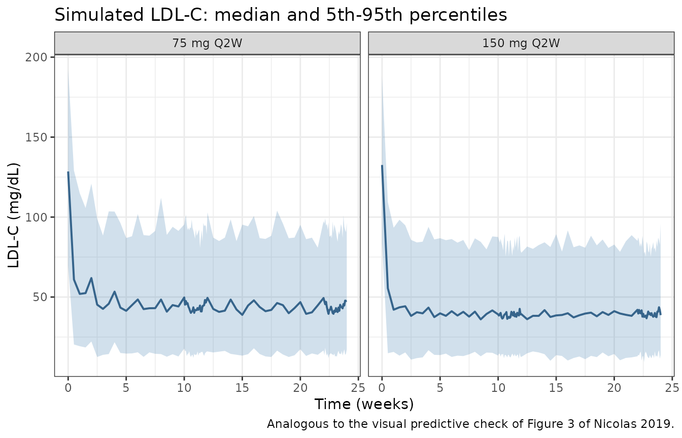

Analogous to Figure 3 of Nicolas 2019: LDL-C vs time by dose arm.

sim |>
  dplyr::group_by(arm, time) |>
  dplyr::summarise(
    Q05 = stats::quantile(Cc, 0.05),
    Q50 = stats::quantile(Cc, 0.50),
    Q95 = stats::quantile(Cc, 0.95),
    .groups = "drop"
  ) |>
  ggplot(aes(time / 7, Q50)) +
  geom_ribbon(aes(ymin = Q05, ymax = Q95), alpha = 0.25, fill = "darkorange") +
  geom_line(colour = "darkorange3", linewidth = 0.7) +
  facet_wrap(~arm) +
  labs(
    x = "Time (weeks)", y = "Total alirocumab (mg/L)",
    title = "Simulated alirocumab exposure (Martinez 2019 Part I PK, fixed)"
  ) +
  theme_bw()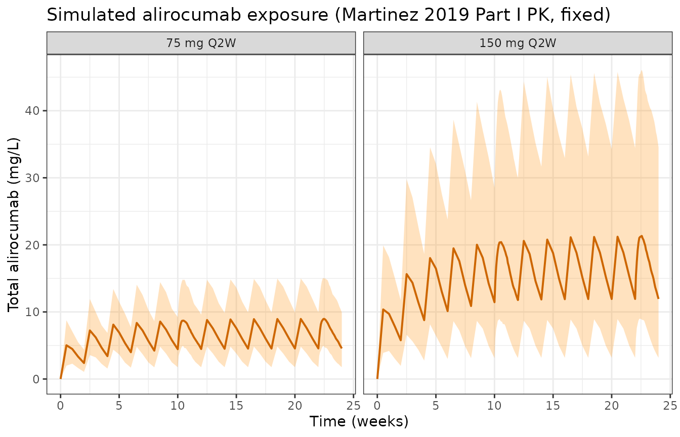

Alirocumab serum concentration driving the PD layer (Part I PK, carried fixed).

derived <- sim |>
  dplyr::filter(time >= 70, time <= 84) |>
  dplyr::group_by(id, arm) |>
  dplyr::summarise(
    base = dplyr::first(LDLC),
    dmax = 100 * (1 - min(ldl) / dplyr::first(LDLC)),
    dtrough = 100 * (1 - ldl[which.max(time)] / dplyr::first(LDLC)),
    SEXF = dplyr::first(SEXF),
    CONMED_STATIN = dplyr::first(CONMED_STATIN),
    .groups = "drop"
  ) |>
  dplyr::mutate(
    Sex = ifelse(SEXF == 1, "Female", "Male"),
    Statin = ifelse(CONMED_STATIN == 1, "Statin", "No statin")
  )

derived |>
  tidyr::pivot_longer(c(dmax, dtrough), names_to = "endpoint", values_to = "pct") |>
  dplyr::mutate(endpoint = ifelse(endpoint == "dmax",
                                  "LDL-C max decrease", "LDL-C decrease at trough")) |>
  ggplot(aes(Sex, pct, fill = arm)) +
  geom_boxplot(outlier.size = 0.5) +
  facet_wrap(~endpoint) +
  labs(
    x = NULL, y = "Decrease from baseline (%)", fill = NULL,
    title = "Derived PD endpoints, weeks 10-12, by sex and dose",
    caption = "Analogous to Figure 4 of Nicolas 2019."
  ) +
  theme_bw()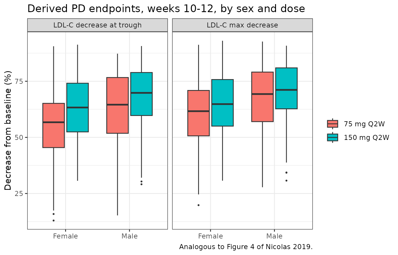

Analogous to Figure 4 of Nicolas 2019: derived endpoints by covariate subgroup.

PKNCA validation

Nicolas 2019 reports no non-compartmental analysis of its own – it is a PD paper that consumes concentrations predicted by Part I. The NCA below therefore characterises the exposure the packaged PK layer delivers over the steady-state dosing interval, and supplies the integral used in the mass-balance gate that follows. PK validation against published alirocumab NCA belongs to the Part I vignette, Martinez_2019_alirocumab.

# Steady-state interval: the dose on day 154 through day 168.
sim_nca <- sim |>
  dplyr::filter(!is.na(Cc), time >= 154, time <= 168) |>
  dplyr::transmute(id, arm, time = time - 154, Cc)

# Guarantee a time-zero record per (id, arm) so PKNCA can anchor the interval.
sim_nca <- dplyr::bind_rows(
  sim_nca,
  sim_nca |>
    dplyr::group_by(id, arm) |>
    dplyr::slice_min(time, n = 1, with_ties = FALSE) |>
    dplyr::ungroup() |>
    dplyr::mutate(time = 0)
) |>
  dplyr::distinct(id, arm, time, .keep_all = TRUE) |>
  dplyr::arrange(id, arm, time)

conc_obj <- PKNCA::PKNCAconc(as.data.frame(sim_nca), Cc ~ time | arm + id)

dose_df <- events |>
  dplyr::filter(evid == 1, time == 154) |>
  dplyr::transmute(id, arm, time = 0, amt)
dose_obj <- PKNCA::PKNCAdose(as.data.frame(dose_df), amt ~ time | arm + id)

intervals <- data.frame(
  start = 0, end = 14,
  cmax = TRUE, tmax = TRUE, cmin = TRUE, auclast = TRUE
)

nca_res <- PKNCA::pk.nca(PKNCA::PKNCAdata(conc_obj, dose_obj, intervals = intervals))

nca_summary <- as.data.frame(nca_res) |>
  dplyr::group_by(arm, PPTESTCD) |>
  dplyr::summarise(median = stats::median(PPORRES), .groups = "drop") |>
  tidyr::pivot_wider(names_from = PPTESTCD, values_from = median)

nca_summary |>
  dplyr::rename(
    "Dose arm" = arm, "Cmax (mg/L)" = cmax, "Tmax (day)" = tmax,
    "Ctrough (mg/L)" = cmin, "AUC0-tau (mg*day/L)" = auclast
  ) |>
  knitr::kable(digits = 2,
               caption = "Simulated steady-state alirocumab exposure (median over 200 subjects per arm), weeks 22-24.")

Simulated steady-state alirocumab exposure (median over 200 subjects per arm), weeks 22-24.
Dose arm	AUC0-tau (mg*day/L)	Cmax (mg/L)	Ctrough (mg/L)	Tmax (day)
150 mg Q2W	243.13	21.51	11.93	4
75 mg Q2W	98.06	9.03	4.56	4


# Exposure must rise with dose, and more than proportionally: alirocumab's
# target-mediated elimination saturates, which is the whole reason Part I
# needed a Michaelis-Menten arm.
auc75 <- nca_summary$auclast[nca_summary$arm == "75 mg Q2W"]
auc150 <- nca_summary$auclast[nca_summary$arm == "150 mg Q2W"]
c(auc_ratio = auc150 / auc75, dose_ratio = 2)
#>  auc_ratio dose_ratio 
#>   2.479449   2.000000
stopifnot(auc150 / auc75 > 2)

Comparison against the published derived endpoints

Table 4 of Nicolas 2019 is the paper’s own validation-grade output: the distribution of the maximum percentage decrease in LDL-C from baseline (DLDL-Cmax) and the percentage decrease at the pre-dose trough (DLDL-Ctrough) within one dosing interval, for phase III patients. The weeks 10-12 window is computed on all patients starting each dose and is the comparator used here; see the caveat below the table for why the weeks 22-24 window is not a like-for-like comparison.

published_t4 <- tibble::tribble(
  ~arm,           ~stat,                  ~published,
  "75 mg Q2W",    "Median LDL-C max decrease (%)",     63.6,
  "75 mg Q2W",    "Median LDL-C trough decrease (%)",  56.4,
  "150 mg Q2W",   "Median LDL-C max decrease (%)",     74.4,
  "150 mg Q2W",   "Median LDL-C trough decrease (%)",  70.8
)

simulated_t4 <- derived |>
  dplyr::group_by(arm) |>
  dplyr::summarise(
    `Median LDL-C max decrease (%)` = stats::median(dmax),
    `Median LDL-C trough decrease (%)` = stats::median(dtrough),
    .groups = "drop"
  ) |>
  tidyr::pivot_longer(-arm, names_to = "stat", values_to = "simulated")

cmp_t4 <- published_t4 |>
  dplyr::left_join(simulated_t4, by = c("arm", "stat")) |>
  dplyr::mutate(difference = simulated - published)

cmp_t4 |>
  dplyr::rename(
    "Dose arm" = arm, "Endpoint" = stat,
    "Nicolas 2019 Table 4" = published, "Simulated" = simulated,
    "Difference (pct points)" = difference
  ) |>
  knitr::kable(digits = 1,
               caption = "Simulated vs published derived PD endpoints, weeks 10-12, phase III patients.")

Simulated vs published derived PD endpoints, weeks 10-12, phase III patients.
Dose arm	Endpoint	Nicolas 2019 Table 4	Simulated	Difference (pct points)
75 mg Q2W	Median LDL-C max decrease (%)	63.6	65.6	2.0
75 mg Q2W	Median LDL-C trough decrease (%)	56.4	60.3	3.9
150 mg Q2W	Median LDL-C max decrease (%)	74.4	69.5	-4.9
150 mg Q2W	Median LDL-C trough decrease (%)	70.8	67.5	-3.3

The one systematic residual is that the simulated separation between the two dose arms is compressed relative to the paper: the published medians differ by 10.8 percentage points on the maximum decrease, the simulated ones by roughly half that. Both caveats below push in exactly that direction. Holding total PCSK9 at a single dose-independent draw per subject removes a real source of dose separation, because the 150 mg arm sustains a higher total-PCSK9 level and TPCSK9 raises Emax; and drawing the covariates independently, when ESM Figure 1 shows them correlated, mixes high- and low-response covariate combinations that in reality travel together. Neither affects the level of the response, which is what the transcription gates catch.

The gate below is deliberately set on the centre of each distribution and on a percentage-point band, not on extremes or on an exact match. Three things put a floor under the achievable agreement, none of them a property of the model: the cohort’s covariates are reconstructed from published percentiles rather than from the real joint distribution; time-varying total PCSK9 is held at a single on-treatment draw per subject because the paper supplies no trajectory for it; and every value in Table 4 is an exact multiple of 1.2%, a quantisation of roughly plus or minus 0.6% in the published numbers themselves.

stopifnot(
  nrow(cmp_t4) == 4L,
  !anyNA(cmp_t4$simulated),
  # Structural: a mis-transcribed Emax, EC50, Hill coefficient or Kout moves
  # these medians by tens of percentage points.
  max(abs(cmp_t4$difference)) < 15,
  # Direction: the model must reproduce the dose separation the paper reports.
  cmp_t4$simulated[cmp_t4$arm == "150 mg Q2W" &
                     cmp_t4$stat == "Median LDL-C max decrease (%)"] >
    cmp_t4$simulated[cmp_t4$arm == "75 mg Q2W" &
                       cmp_t4$stat == "Median LDL-C max decrease (%)"],
  # The trough decrease is always smaller than the peak decrease, per arm.
  all(
    cmp_t4$simulated[cmp_t4$stat == "Median LDL-C trough decrease (%)"] <
      cmp_t4$simulated[cmp_t4$stat == "Median LDL-C max decrease (%)"]
  )
)

The cohort spread is also worth comparing against the paper’s own, since the PD inter-individual variability (Emax CV 64.8%) is what produces it:

spread <- derived |>
  dplyr::group_by(arm) |>
  dplyr::summarise(
    `5th pct` = stats::quantile(dmax, 0.05),
    Median = stats::median(dmax),
    `95th pct` = stats::quantile(dmax, 0.95),
    .groups = "drop"
  ) |>
  dplyr::mutate(
    `Published 5th pct` = ifelse(arm == "75 mg Q2W", 32.4, 45.6),
    `Published median` = ifelse(arm == "75 mg Q2W", 63.6, 74.4),
    `Published 95th pct` = ifelse(arm == "75 mg Q2W", 82.8, 88.8)
  )

spread |>
  dplyr::rename("Dose arm" = arm) |>
  knitr::kable(digits = 1,
               caption = "LDL-C maximum decrease, weeks 10-12: simulated vs published 5th / 50th / 95th percentiles.")

LDL-C maximum decrease, weeks 10-12: simulated vs published 5th / 50th / 95th percentiles.
Dose arm	5th pct	Median	95th pct	Published 5th pct	Published median	Published 95th pct
75 mg Q2W	40.3	65.6	86.3	32.4	63.6	82.8
150 mg Q2W	43.3	69.5	87.4	45.6	74.4	88.8


# Robust-quantile envelope, not an extreme: the 95th percentile of a saturating
# response is bounded above by 100 * Emax/(1+Emax) and both sides sit near it.
stopifnot(all(abs(spread$`95th pct` - spread$`Published 95th pct`) < 15))

Assumptions and deviations

kin is derived, not published. Nicolas 2019 Table 2 reports Kout, EC50, Emax and the Hill coefficient, and no production rate or typical baseline. The model file sets kin = kout * LDLC from the drug-free steady state of the type IV indirect response model, with LDLC the subject’s own observed pre-treatment value – the reading that is consistent with the paper screening “baseline LDL-C” as a covariate and with it reporting all derived endpoints as percentages. Structural checks 1 and 2 verify that the state holds exactly at baseline without drug and that the percentage profile is exactly independent of the baseline, so the choice changes no percentage the paper publishes.
The PK layer is inherited, not fitted here. Every PK ini() entry comes from Martinez 2019 (Part I) Table 2 and is wrapped in fixed(). Part II used individual (empirical Bayes) PK parameters from Part I; this packaged model necessarily uses the Part I population model with its inter-individual variability instead, which reproduces the exposure distribution but not any particular subject’s Part I post hoc estimates.
The Part I covariate effects are held at their reference values. Part II re-estimated nothing in the PK layer, so body weight, age, statin use and free PCSK9 do not act on the PK here even though they do in Martinez_2019_alirocumab. A user who needs covariate-dependent exposure should drive the Part I model directly and feed its concentrations in.
Alirocumab concentration carries no residual error. Part II consumed Part I predictions (Sect. 2.4), so Cc is an algebraic observable here and the only endpoint with a residual error model is ldl. The Part I residual error parameters are therefore not carried.
Time-varying total PCSK9 is supplied, not generated. TPCSK9 is a model input: the packaged model has no PCSK9 state. The vignette holds it at one on-treatment draw per subject from the published 5th/50th/95th percentiles (491 / 3340 / 6340 ng/mL). In reality it rises from its pre-treatment level over the first weeks of dosing, so the early part of the simulated profile slightly overstates Emax; the endpoint windows this vignette gates on (weeks 10-12) are well past that transient. A user wanting the trajectory can take the total_target state of Djebli_2017_alirocumab.
Baseline LDL-C is not published and is drawn uniformly over 100-160 mg/dL. It affects only the absolute mg/dL axis of the profile figure; structural check 2 proves it cancels from every percentage endpoint.
Covariate distributions are reconstructed from published percentiles by piecewise-linear quantile interpolation through the 5th / 50th / 95th values in Sect. 3.5 and Sect. 4, restricted to that range. The paper publishes no joint distribution and no correlation structure, so the covariates are drawn independently; ESM Figure 1 shows they are in fact correlated (the scatterplot matrix of continuous covariates), which is the main reason the simulated spread is not expected to match the published spread exactly.
No up-titration is simulated. In the phase III programme the 75 mg Q2W dose could be increased to 150 mg Q2W at week 12 for inadequate responders. That is why the paper’s weeks 22-24 statistics for the 75 mg arm (median max decrease 68.4%) are higher than its weeks 10-12 statistics (63.6%): the later window contains only the patients who did not need an increase, an enriched responder subgroup. This vignette gates on the weeks 10-12 window, which the paper computes on all patients starting each dose, and does not compare the weeks 22-24 window at all.

Errata and source inconsistencies

Recorded because each one is a place where a careful transcription could reasonably have gone the other way.

The Sect. 3.2 displayed Emax equation misprints one coefficient. It shows the total-PCSK9 slope as 0.0003331; Table 2, the Table 2 footnote c, the bootstrap column (0.000328, 95% CI 0.000266-0.000418) and all twelve ESM Table 3 cells agree on 0.000331. The model uses 0.000331. With the extra digit, the ESM Table 3 cell for the 5th-percentile TPCSK9 in women computes as 1.04 against a published 1.05.
The Emax parenthesisation is decided by ESM Table 3, not by the narrative. The printed equation puts the free-baseline-PCSK9 and statin terms outside the multiplicative sex / age / weight chain, and all twelve ESM Table 3 cells reproduce on that reading to three significant figures – decisively so in the female-plus-statin column (published 1.45 / 2.12 / 2.81 against 1.45 / 2.12 / 2.81 computed; a sex-outermost reading would give 1.33 / 2.00 / 2.69). Sect. 3.5’s free-baseline-PCSK9 Emax ranges are the one place that disagrees: it reports 1.56-2.62 at the 5th percentile and 1.97-3.21 at the 95th, whose lower ends are 1.49 and 2.08 on the printed equation but exactly 1.56 and 1.97 if the additive terms are moved inside the sex factor. The two printed equations plus twelve ESM cells outweigh two narrative numbers, so the model follows the printed form. The accompanying “20.9 to 26.4%” impact statement reconciles with neither reading (the printed form gives 39.2% and 22.3%).
The Emax inter-individual variability is printed twice, differently. Table 2 gives 0.420 (65.8) while Sect. 3.4 says 64.8%. sqrt(0.420) = 0.648, so 64.8% is correct and the table’s 65.8 is a typographical error. The model transcribes the variance 0.420 directly, so nothing propagates. The same identity confirms that the parenthesised percentages in Table 2 are 100 * sqrt(variance) and not 100 * sqrt(exp(variance) - 1): 0.113, 0.123 and 0.296 give 33.6, 35.1 and 54.4 against the tabulated 33.7, 35.1 and 54.4.
The Emax row’s 95% confidence interval in Table 2 is a duplicate. It reads 1.63-1.92, which is the Hill-coefficient row’s interval; the Emax point estimate 2.43 lies outside it. The bootstrap column gives 2.24-2.91, which does contain it. No model value depends on either.
Every value in Table 4 is an exact multiple of 1.2%. All 32 tabulated percentages – medians, means, percentiles and extremes alike – are multiples of 1.2, which bounds the precision of any comparison against that table at roughly plus or minus 0.6 percentage points.
Kout is a two-level switch, not a reference value with a shift. Table 2’s “Typical value of Kout” (0.00395 /h) is the healthy-volunteer level and the “Effect of DISST on Kout” row (0.00997 /h) is the patient level in full, per footnote a. Reading the second row as an increment would give a patient Kout of 0.0139 /h, 40% too fast.
The two halves of the analysis define CONMED_STATIN differently. Part I (Martinez 2019) counts only rosuvastatin below 20 mg/day, atorvastatin below 40 mg/day and simvastatin at any dose; Part II counts any statin at any dose. The same column name therefore carries different memberships in the two model files and a data set must be built per model.
Nicolas 2019 is Part II of a pair. The companion Part I popPK paper (Martinez 2019, doi:10.1007/s40262-018-0669-y) is packaged separately as Martinez_2019_alirocumab; a third alirocumab model from the same group (Djebli 2017, a quasi-steady-state TMDD model that also carries total PCSK9 as a state) is packaged as Djebli_2017_alirocumab.