Tacrolimus with voriconazole co-therapy (Zhao 2024)
Source:vignettes/articles/Zhao_2024_tacrolimus.Rmd
Zhao_2024_tacrolimus.RmdModel and source
mod <- readModelDb("Zhao_2024_tacrolimus")
ui  <- rxode2::rxode(mod)
#> ℹ parameter labels from comments will be replaced by 'label()'- Citation: Zhao Y-C, Sun Z-H, Li J-K, Liu H-Y, Zhang B-K, Xie X-B, Fang C-H, Sandaradura I, Peng F-H, Yan M. Individualized dosing parameters for tacrolimus in the presence of voriconazole: a real-world PopPK study. Front Pharmacol. 2024;15:1439232. doi:10.3389/fphar.2024.1439232. Parameter values are the final-model estimates in Table 3 (‘Final model’ block), cross-checked against the bootstrap summary in Table 4.
- Article: https://doi.org/10.3389/fphar.2024.1439232
- Description: One-compartment population PK model with first-order absorption for oral tacrolimus in adult renal transplant recipients co-administered voriconazole, built from within-15-days-post-transplant therapeutic drug monitoring. The absorption rate constant is fixed and the residual error is additive because the data are almost entirely troughs. Apparent clearance and apparent volume of distribution both fall as the measured voriconazole concentration rises (CYP3A4 inhibition), and apparent clearance also falls as serum creatinine rises.
Zhao 2024 develops a single population PK model, so this paper contributes one model file.
Population
The model was built on a retrospective, non-interventional single-centre cohort of 19 adult first-time renal transplant recipients treated at The Second Xiangya Hospital of Central South University, Changsha, China, between January 2016 and March 2021 (ChiCTR2100048712). Every patient received oral tacrolimus as part of a triple immunosuppressive regimen (with mycophenolate mofetil and a glucocorticoid) and started voriconazole within 15 days of transplantation.
Baseline characteristics (Zhao 2024 Table 1): 15/19 male (78.9%); median age 44 years (IQR 37.5-52.5); median weight 63 kg (IQR 51-72); median tacrolimus dose 3.00 mg per administration (IQR 1.50-3.50); median observed tacrolimus concentration 7.90 ng/mL (IQR 5.55-10.78); median time after operation 8 days (IQR 4-11); median voriconazole concentration 0.00 ug/mL (IQR 0.00-0.50) with an observed range of 0-3.38 ug/mL; median serum creatinine 237 umol/L (IQR 162.9-648.0). CYP3A5 genotyping was an inclusion requirement, but only *1/*3 (n = 10) and *3/*3 (n = 9) carriers were enrolled – no *1/*1 – and neither CYP3A5 nor CYP2C19 genotype survived covariate selection.
167 whole-blood tacrolimus concentrations were collected (8-9 per patient), the majority within 30 minutes before a dose, so the dataset is dominated by troughs. That is why Ka had to be fixed and why an additive residual model was selected.
The same information is available programmatically from
rxode2::rxode(readModelDb("Zhao_2024_tacrolimus"))$population.
Source trace
Per-parameter origins are recorded as in-file comments beside each
ini() entry; they are collected here for review. Zhao 2024
prints no display equations at all – neither the
structural model nor the covariate model – so the functional forms below
were reconstructed from the Table 3 and Table 4 footnotes (“exponent for
<covariate>, as a covariate for
<parameter>”), from the covariate distributions in
Table 1, and from the simulation settings stated in section 3.4. This is
documented in full under Assumptions and deviations.
| Quantity | Value | Source location |
|---|---|---|
| Structural model: one compartment, first-order absorption and elimination | n/a | Section 3.2.1, “a one-compartment model with first-order absorption and elimination … was selected” |
| Residual model: additive | n/a | Section 3.2.1, “along with an additive residual model”; Table 2
model-comparison row 1a_Addictive
|
Ka (fixed) |
8.39 1/h | Table 3, final model row Ka; fixed status from Table 3
base-model row Ka (Fixed) (Stderr 0.00, CI 8.39-8.39) and
from the Discussion, “the Ka value was fixed during the model’s
development” |
V/F |
2690 L | Table 3, final model row V/F; bootstrap mean 2655, 95%
CI 1480-4060 (Table 4 tvV) |
CL/F |
42.87 L/h | Table 3, final model row CL/F; bootstrap mean 42.00,
95% CI 30-50 (Table 4 tvCl) |
| Voriconazole coefficient on CL/F | -0.28 | Table 3 / Table 4 row Theta VRC-CL (Stderr 0.03;
bootstrap 95% CI -0.99 to -0.21) |
| Voriconazole coefficient on V/F | -0.20 | Table 3 / Table 4 row Theta VRC-V (Stderr 0.04;
bootstrap 95% CI -0.36 to -0.03) |
| Serum-creatinine exponent | -0.40 | Table 3 / Table 4 row Theta CREA-V (Stderr 0.11;
bootstrap 95% CI -0.72 to -0.05) |
| Serum-creatinine normalising constant, 237 umol/L | n/a | Table 1 cohort median; section 3.4.1, “The CREA value, fixed at the median of 237 umol/L” |
omega^2 V |
0.02 | Table 4, row omega 2 V
|
omega^2 CL |
0.16 | Table 4, row omega 2 CL
|
sigma (additive) |
3.50 ng/mL | Table 4, row sigma; bootstrap mean 3.41, 95% CI
3.06-3.74 |
Structural verification against the closed form
With the random effects zeroed, the one-compartment first-order-absorption model has an exact closed form, so a solve of the rxode2 model must reproduce superposition of single-dose profiles to numerical precision. This check has no random component, so a tight bound is the correct assertion here.
typ <- rxode2::zeroRe(mod)
#> ℹ parameter labels from comments will be replaced by 'label()'

kaRef   <- 8.39
clRef   <- 42.87
vcRef   <- 2690
doseMg  <- 3
dosingT <- seq(0, 60, by = 12)   # q12h for 3 days: 6 doses
obsT    <- seq(0, 84, by = 0.5)

evTyp <-
  dplyr::bind_rows(
    data.frame(id = 1L, time = dosingT, amt = doseMg, evid = 1L,
               cmt = "depot", dv = NA_real_),
    data.frame(id = 1L, time = obsT, amt = NA_real_, evid = 0L,
               cmt = "central", dv = NA_real_)
  ) |>
  dplyr::mutate(CONC_VORI_NGML = 0, CREAT = 237) |>
  dplyr::arrange(time, dplyr::desc(evid))

simTyp <- rxode2::rxSolve(typ, evTyp, returnType = "data.frame")
#> ℹ omega/sigma items treated as zero: 'etalvc', 'etalcl'

# Closed-form superposition, in ng/mL (dose mg / volume L = mg/L = 1000 ng/mL)
singleDose <- function(tau, dose, ka, cl, vc) {
  kel <- cl / vc
  out <- 1000 * dose * ka / (vc * (ka - kel)) * (exp(-kel * tau) - exp(-ka * tau))
  ifelse(tau < 0, 0, out)
}
closed <- vapply(
  simTyp$time,
  function(tt) sum(singleDose(tt - dosingT, doseMg, kaRef, clRef, vcRef)),
  numeric(1)
)

relDiff <- abs(simTyp$Cc - closed) / pmax(closed, 1e-8)
summary(relDiff)
#>      Min.   1st Qu.    Median      Mean   3rd Qu.      Max.
#> 0.000e+00 2.667e-07 2.920e-07 3.456e-07 4.425e-07 6.345e-07

stopifnot(max(relDiff) < 1e-3)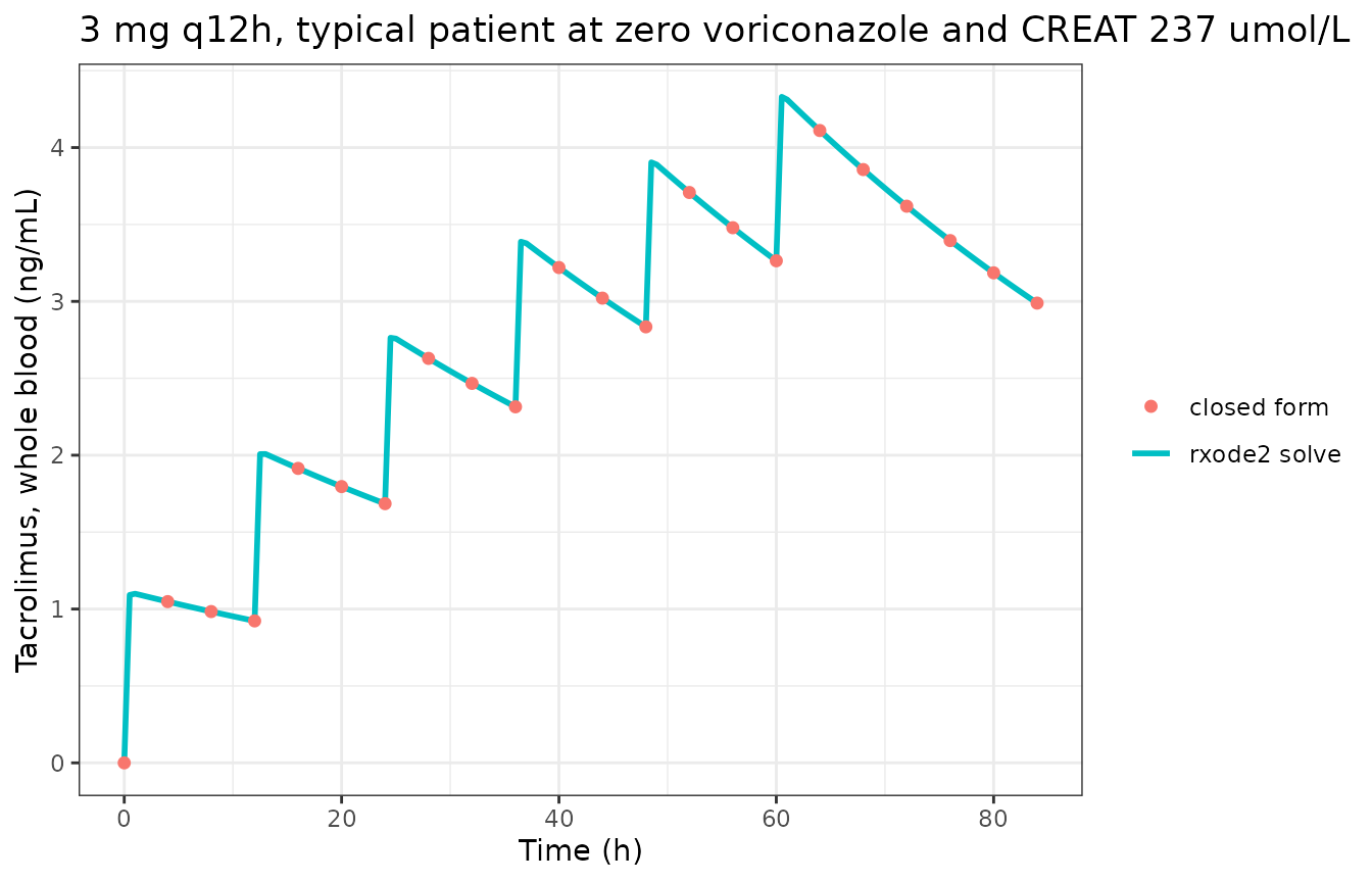
Covariate effects: replicating the published dose-recommendation simulations
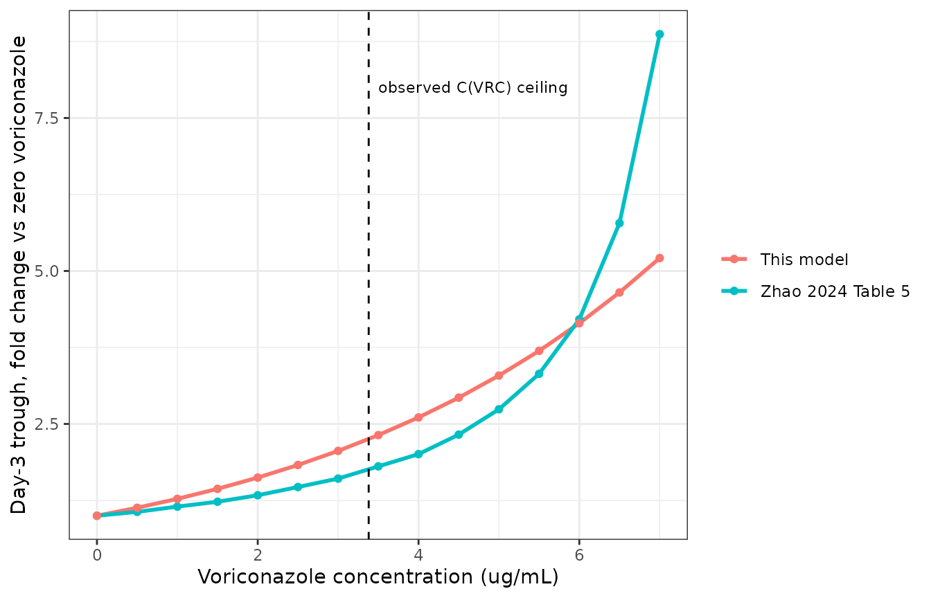
Zhao 2024 sections 3.4.1 and 3.4.2 report Monte Carlo simulations of the day-3 trough (72 h after the first dose, on a q12h schedule, i.e. after six doses) across a grid of voriconazole concentrations at fixed CREA = 237 umol/L (Table 5) and across a grid of serum creatinines at fixed voriconazole = 0 (Table 6).
day3Trough <- function(cvrcUgMl, creat, doseMg) {
  ev <-
    dplyr::bind_rows(
      data.frame(time = dosingT, amt = doseMg, evid = 1L, cmt = "depot"),
      data.frame(time = 72,      amt = NA_real_, evid = 0L, cmt = "central")
    ) |>
    dplyr::mutate(id = 1L,
                  CONC_VORI_NGML = cvrcUgMl * 1000,
                  CREAT = creat) |>
    dplyr::arrange(time, dplyr::desc(evid))
  out <- rxode2::rxSolve(typ, ev, returnType = "data.frame")
  out$Cc[out$time == 72][1]
}
Voriconazole concentration (Zhao 2024 Table 5)
vGrid <- c(0, 0.5, 1, 1.5, 2, 2.5, 3, 3.5, 4, 4.5, 5, 5.5, 6, 6.5, 7)
# Published Table 5, tacrolimus 5.5 mg q12h column (mean day-3 trough, ng/mL)
table5Pub <- c(9.06, 9.63, 10.41, 11.13, 12.09, 13.31, 14.56, 16.37,
               18.18, 21.07, 24.82, 30.07, 38.14, 52.39, 80.36)

table5 <- data.frame(
  cvrc      = vGrid,
  published = table5Pub,
  model     = vapply(vGrid, day3Trough, numeric(1), creat = 237, doseMg = 5.5)
) |>
  dplyr::mutate(
    pubFold   = published / published[1],
    modelFold = model / model[1]
  )
#> ℹ omega/sigma items treated as zero: 'etalvc', 'etalcl'
#> ℹ omega/sigma items treated as zero: 'etalvc', 'etalcl'
#> ℹ omega/sigma items treated as zero: 'etalvc', 'etalcl'
#> ℹ omega/sigma items treated as zero: 'etalvc', 'etalcl'
#> ℹ omega/sigma items treated as zero: 'etalvc', 'etalcl'
#> ℹ omega/sigma items treated as zero: 'etalvc', 'etalcl'
#> ℹ omega/sigma items treated as zero: 'etalvc', 'etalcl'
#> ℹ omega/sigma items treated as zero: 'etalvc', 'etalcl'
#> ℹ omega/sigma items treated as zero: 'etalvc', 'etalcl'
#> ℹ omega/sigma items treated as zero: 'etalvc', 'etalcl'
#> ℹ omega/sigma items treated as zero: 'etalvc', 'etalcl'
#> ℹ omega/sigma items treated as zero: 'etalvc', 'etalcl'
#> ℹ omega/sigma items treated as zero: 'etalvc', 'etalcl'
#> ℹ omega/sigma items treated as zero: 'etalvc', 'etalcl'
#> ℹ omega/sigma items treated as zero: 'etalvc', 'etalcl'

knitr::kable(
  table5 |>
    dplyr::rename(
      "Voriconazole (ug/mL)"    = cvrc,
      "Published (ng/mL)"       = published,
      "This model (ng/mL)"      = model,
      "Published fold vs 0"     = pubFold,
      "This model fold vs 0"    = modelFold
    ),
  digits = 2,
  caption = "Replicates Zhao 2024 Table 5, 5.5 mg q12h column: day-3 trough vs voriconazole concentration at CREA = 237 umol/L."
)| Voriconazole (ug/mL) | Published (ng/mL) | This model (ng/mL) | Published fold vs 0 | This model fold vs 0 |
|---|---|---|---|---|
| 0.0 | 9.06 | 6.63 | 1.00 | 1.00 |
| 0.5 | 9.63 | 7.50 | 1.06 | 1.13 |
| 1.0 | 10.41 | 8.46 | 1.15 | 1.28 |
| 1.5 | 11.13 | 9.55 | 1.23 | 1.44 |
| 2.0 | 12.09 | 10.77 | 1.33 | 1.62 |
| 2.5 | 13.31 | 12.13 | 1.47 | 1.83 |
| 3.0 | 14.56 | 13.66 | 1.61 | 2.06 |
| 3.5 | 16.37 | 15.38 | 1.81 | 2.32 |
| 4.0 | 18.18 | 17.29 | 2.01 | 2.61 |
| 4.5 | 21.07 | 19.44 | 2.33 | 2.93 |
| 5.0 | 24.82 | 21.83 | 2.74 | 3.29 |
| 5.5 | 30.07 | 24.51 | 3.32 | 3.69 |
| 6.0 | 38.14 | 27.50 | 4.21 | 4.15 |
| 6.5 | 52.39 | 30.84 | 5.78 | 4.65 |
| 7.0 | 80.36 | 34.57 | 8.87 | 5.21 |
# Direction and monotonicity are reproduced exactly; absolute levels are not.
stopifnot(
  all(diff(table5$model) > 0),
  table5$model[table5$cvrc == 0] > 0
)
The model reproduces the direction and the monotonicity of Table 5, but not its absolute level: the published day-3 troughs run about 1.4 times higher than the model at zero voriconazole, and the published curve is flatter than the model over the observed 0-3.38 ug/mL range and steeper above it. This is a property of the published table, not of the extraction – see Assumptions and deviations. No parameter has been tuned to close the gap.
Serum creatinine (Zhao 2024 Table 6)
cGrid <- c(40, 100, 160, 400, 600, 800, 1000, 1600, 1800, 2000)
# Published Table 6, tacrolimus 5.5 mg q12h row (mean day-3 trough, ng/mL)
table6Pub <- c(6.46, 8.58, 9.73, 12.42, 13.32, 14.16, 14.44, 15.46, 15.94, 15.60)

table6 <- data.frame(
  creat     = cGrid,
  published = table6Pub,
  model     = vapply(cGrid, function(cc) day3Trough(0, cc, 5.5), numeric(1))
) |>
  dplyr::mutate(
    pubFold   = published / published[1],
    modelFold = model / model[1]
  )
#> ℹ omega/sigma items treated as zero: 'etalvc', 'etalcl'
#> ℹ omega/sigma items treated as zero: 'etalvc', 'etalcl'
#> ℹ omega/sigma items treated as zero: 'etalvc', 'etalcl'
#> ℹ omega/sigma items treated as zero: 'etalvc', 'etalcl'
#> ℹ omega/sigma items treated as zero: 'etalvc', 'etalcl'
#> ℹ omega/sigma items treated as zero: 'etalvc', 'etalcl'
#> ℹ omega/sigma items treated as zero: 'etalvc', 'etalcl'
#> ℹ omega/sigma items treated as zero: 'etalvc', 'etalcl'
#> ℹ omega/sigma items treated as zero: 'etalvc', 'etalcl'
#> ℹ omega/sigma items treated as zero: 'etalvc', 'etalcl'

knitr::kable(
  table6 |>
    dplyr::rename(
      "Serum creatinine (umol/L)" = creat,
      "Published (ng/mL)"         = published,
      "This model (ng/mL)"        = model,
      "Published fold vs 40"      = pubFold,
      "This model fold vs 40"     = modelFold
    ),
  digits = 2,
  caption = "Replicates Zhao 2024 Table 6, 5.5 mg q12h row: day-3 trough vs serum creatinine at zero voriconazole."
)| Serum creatinine (umol/L) | Published (ng/mL) | This model (ng/mL) | Published fold vs 40 | This model fold vs 40 |
|---|---|---|---|---|
| 40 | 6.46 | 3.89 | 1.00 | 1.00 |
| 100 | 8.58 | 5.30 | 1.33 | 1.36 |
| 160 | 9.73 | 6.04 | 1.51 | 1.55 |
| 400 | 12.42 | 7.39 | 1.92 | 1.90 |
| 600 | 13.32 | 7.94 | 2.06 | 2.04 |
| 800 | 14.16 | 8.30 | 2.19 | 2.13 |
| 1000 | 14.44 | 8.57 | 2.24 | 2.20 |
| 1600 | 15.46 | 9.09 | 2.39 | 2.34 |
| 1800 | 15.94 | 9.22 | 2.47 | 2.37 |
| 2000 | 15.60 | 9.32 | 2.41 | 2.39 |
foldRatio <- table6$modelFold[length(cGrid)] / table6$pubFold[length(cGrid)]
foldRatio
#> [1] 0.9916664

stopifnot(
  # Monotone increase in serum creatinine, as the paper reports.
  all(diff(table6$model) > 0),
  # The 40 -> 2000 umol/L fold-rise matches the published table within 10%.
  abs(foldRatio - 1) < 0.10,
  # Every intermediate fold-change is within 10% of the published fold-change.
  max(abs(table6$modelFold / table6$pubFold - 1)) < 0.10
)
Placing the -0.40 exponent on CL/F reproduces the published Table 6 fold-change profile closely: over the full 40-2000 umol/L grid the model predicts a 2.39-fold rise in day-3 trough against the published 2.41-fold, and every intermediate point agrees within 10%. Placing the same exponent on V/F instead gives only a 1.80-fold rise at 72 h and inverts the direction entirely by the time steady state is approached, so it cannot generate Table 6. See Assumptions and deviations – the paper is internally inconsistent about which parameter this coefficient modifies.
Simulated cohort
A 100-subject cohort at the cohort-median covariates, dosed 3 mg q12h, with the published inter-individual and residual variability.
rxode2::rxSetSeed(20240910)
nSub <- 100L

evCohort <-
  dplyr::bind_rows(
    tidyr::expand_grid(id = seq_len(nSub), time = dosingT) |>
      dplyr::mutate(amt = doseMg, evid = 1L, cmt = "depot"),
    tidyr::expand_grid(id = seq_len(nSub), time = seq(0, 84, by = 2)) |>
      dplyr::mutate(amt = NA_real_, evid = 0L, cmt = "central")
  ) |>
  dplyr::mutate(CONC_VORI_NGML = 0, CREAT = 237) |>
  dplyr::arrange(id, time, dplyr::desc(evid))

simCohort <- rxode2::rxSolve(mod, evCohort, returnType = "data.frame")
#> ℹ parameter labels from comments will be replaced by 'label()'

at72 <- dplyr::filter(simCohort, time == 72)

# ipredSim is the individual prediction (inter-individual variability only);
# sim additionally carries the additive residual error.
rbind(
  ipred = quantile(at72$ipredSim, c(0.05, 0.25, 0.5, 0.75, 0.95)),
  sim   = quantile(at72$sim,      c(0.05, 0.25, 0.5, 0.75, 0.95))
)
#>              5%      25%     50%      75%      95%
#> ipred  2.313409 3.086776 3.81256 4.199064 4.956764
#> sim   -1.156809 1.699948 4.12033 6.293366 8.600039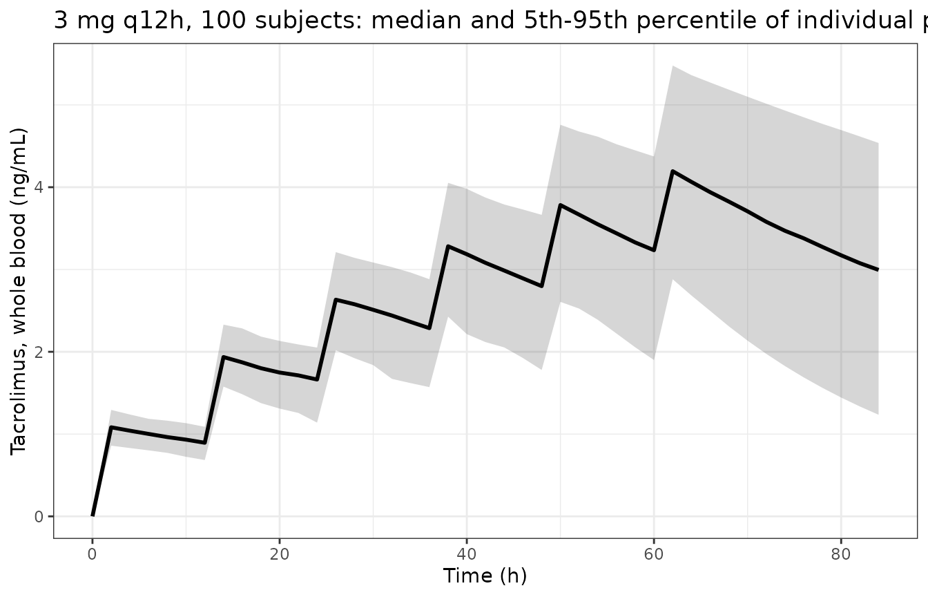
Two things are worth stating plainly here rather than glossed over.
The additive residual drives simulated observations
negative. With sigma = 3.50 ng/mL and a typical
day-3 trough of about 3.6 ng/mL at 3 mg q12h, the lower tail of
sim is below zero. That is an inherent consequence of an
additive error model fitted to a variable whose typical value is
single-digit ng/mL, not an extraction error – the paper reports exactly
this sigma against a median observed concentration of 7.90 ng/mL, and
its own Discussion flags the residual as unexpectedly large. Users
simulating observations from this model should truncate at zero.
The model’s day-3 trough runs below the cohort’s observed concentrations. At the cohort-median dose of 3 mg q12h the model predicts a day-3 trough near 3.6 ng/mL, against a median observed tacrolimus concentration of 7.90 ng/mL in Table 1. Part of that gap is timing – the observed samples have a median of 8 days post-operation, closer to steady state than day 3, and the model’s steady-state trough at the same dose is about 5.3 ng/mL – and part of it is the same systematic offset that separates this model from the paper’s own Table 5 and Table 6 (see Errata). Nothing has been adjusted to close it.
kelRef <- clRef / vcRef
ssTrough <- 1000 * doseMg / vcRef * kaRef / (kaRef - kelRef) *
  (exp(-kelRef * 12) / (1 - exp(-kelRef * 12)) -
     exp(-kaRef * 12) / (1 - exp(-kaRef * 12)))

c(day3Typical       = day3Trough(0, 237, doseMg),
  steadyStateTypical = ssTrough,
  cohortMedianIpred  = median(at72$ipredSim),
  cohortObservedMedian = 7.90)
#> ℹ omega/sigma items treated as zero: 'etalvc', 'etalcl'
#>          day3Typical   steadyStateTypical    cohortMedianIpred
#>             3.618766             5.301796             3.812560
#> cohortObservedMedian
#>             7.900000

stopifnot(
  # Centre of the individual-prediction distribution, with headroom on both
  # sides; deliberately not an assertion on the tails, which are not stable
  # across rxode2 builds.
  median(at72$ipredSim) > 2,
  median(at72$ipredSim) < 6
)
PKNCA validation
Zhao 2024 reports no non-compartmental analysis, so there is no
published Cmax / Tmax / AUC / half-life table to compare against. The
NCA is therefore used as an internal-identity check: for a single oral
dose of a linear one-compartment model with no residual error, PKNCA
must recover AUC(0-inf) = Dose / (CL/F) and
t(1/2) = ln(2) * (V/F) / (CL/F) for each voriconazole
level, which independently confirms that the covariate terms are wired
onto the parameters the model file claims.
ncaArms <- data.frame(
  treatment = c("C(VRC) 0 ug/mL", "C(VRC) 1 ug/mL", "C(VRC) 2 ug/mL"),
  cvrc      = c(0, 1, 2)
)
ncaDose <- 5

ncaTimes <- sort(unique(c(seq(0, 4, by = 0.1), seq(4, 24, by = 1),
                          seq(24, 480, by = 6))))

evNca <-
  ncaArms |>
  dplyr::rowwise() |>
  dplyr::reframe(
    treatment = treatment,
    cvrc      = cvrc,
    dplyr::bind_rows(
      data.frame(time = 0,        amt = ncaDose,   evid = 1L, cmt = "depot"),
      data.frame(time = ncaTimes, amt = NA_real_,  evid = 0L, cmt = "central")
    )
  ) |>
  dplyr::mutate(
    id             = as.integer(factor(treatment)),
    CONC_VORI_NGML = cvrc * 1000,
    CREAT          = 237
  ) |>
  dplyr::arrange(id, time, dplyr::desc(evid))

simNca <- rxode2::rxSolve(typ, evNca, returnType = "data.frame") |>
  dplyr::left_join(
    dplyr::distinct(evNca, id, treatment, cvrc),
    by = "id"
  )
#> ℹ omega/sigma items treated as zero: 'etalvc', 'etalcl'
#> Warning: multi-subject simulation without without 'omega'

concData <- simNca |>
  dplyr::filter(!is.na(Cc)) |>
  dplyr::select(id, treatment, time, Cc)

doseData <- concData |>
  dplyr::distinct(id, treatment) |>
  dplyr::mutate(time = 0, dose_mg = ncaDose)

ncaIntervals <- data.frame(
  start = 0, end = Inf,
  cmax = TRUE, tmax = TRUE, auclast = TRUE,
  aucinf.obs = TRUE, half.life = TRUE
)

ncaRes <- PKNCA::pk.nca(
  PKNCA::PKNCAdata(
    PKNCA::PKNCAconc(concData, Cc ~ time | treatment + id),
    PKNCA::PKNCAdose(doseData, dose_mg ~ time | treatment + id),
    intervals = ncaIntervals
  )
)

ncaWide <- as.data.frame(ncaRes) |>
  dplyr::select(treatment, PPTESTCD, PPORRES) |>
  tidyr::pivot_wider(names_from = PPTESTCD, values_from = PPORRES)

expected <- ncaArms |>
  dplyr::mutate(
    clExp = 42.87 * exp(-0.28 * cvrc),
    vcExp = 2690 * exp(-0.20 * cvrc),
    aucExp = 1000 * ncaDose / clExp,        # mg/L*h -> ng/mL*h
    thalfExp = log(2) * vcExp / clExp
  )

ncaCompare <- ncaWide |>
  dplyr::left_join(expected, by = "treatment") |>
  dplyr::mutate(
    aucPctDiff   = 100 * (aucinf.obs - aucExp) / aucExp,
    thalfPctDiff = 100 * (half.life - thalfExp) / thalfExp
  )

knitr::kable(
  ncaCompare |>
    dplyr::select(treatment, cmax, tmax, aucinf.obs, aucExp, aucPctDiff,
                  half.life, thalfExp, thalfPctDiff) |>
    dplyr::rename(
      "Arm"                       = treatment,
      "Cmax (ng/mL)"              = cmax,
      "Tmax (h)"                  = tmax,
      "AUC0-inf NCA (ng/mL*h)"    = aucinf.obs,
      "AUC0-inf Dose/CL"          = aucExp,
      "AUC % diff"                = aucPctDiff,
      "t1/2 NCA (h)"              = half.life,
      "t1/2 ln2*V/CL (h)"         = thalfExp,
      "t1/2 % diff"               = thalfPctDiff
    ),
  digits = 2,
  caption = "Single 5 mg oral dose: PKNCA against the model's own closed-form AUC and half-life at three voriconazole concentrations."
)| Arm | Cmax (ng/mL) | Tmax (h) | AUC0-inf NCA (ng/mL*h) | AUC0-inf Dose/CL | AUC % diff | t1/2 NCA (h) | t1/2 ln2*V/CL (h) | t1/2 % diff |
|---|---|---|---|---|---|---|---|---|
| C(VRC) 0 ug/mL | 1.84 | 0.8 | 116.62 | 116.63 | -0.01 | 43.49 | 43.49 | 0 |
| C(VRC) 1 ug/mL | 2.24 | 0.8 | 154.30 | 154.32 | -0.01 | 47.12 | 47.12 | 0 |
| C(VRC) 2 ug/mL | 2.74 | 0.8 | 204.16 | 204.18 | -0.01 | 51.04 | 51.04 | 0 |
stopifnot(
  max(abs(ncaCompare$aucPctDiff)) < 1,
  max(abs(ncaCompare$thalfPctDiff)) < 1,
  # Exposure rises with voriconazole, as the paper reports.
  all(diff(ncaCompare$aucinf.obs) > 0)
)
Both identities hold to well under 1%, and AUC rises monotonically
with voriconazole concentration, confirming that
e_conc_vori_ngml_cl and e_conc_vori_ngml_vc
act on CL/F and V/F respectively and in the direction the paper
reports.
Assumptions and deviations
The paper prints no equations. Zhao 2024 contains no
display equations of any kind – not for the structural model, not for
the random-effect model, not for the covariate model. The only
description of the covariate functional forms is the Table 3 and Table 4
footnote wording, “exponent for <covariate>, as a
covariate for <parameter>”. Everything below follows
from that wording plus the covariate distributions in Table 1 and the
simulation settings in section 3.4. None of it is tuned to a target.
Voriconazole enters exponentially, not as a power. The cohort median voriconazole concentration is exactly 0.00 ug/mL (Table 1) and many samples were drawn before voriconazole was started, so no
(C_VRC / median)^thetaform exists. The model usesexp(theta * C_VRC), which equals 1 atC_VRC = 0– the untreated reference – and is the only Phoenix NLME continuous-covariate form compatible with a zero-valued covariate.Serum creatinine enters as a power normalised to 237 umol/L. CREAT is strictly positive, the footnote calls the coefficient an exponent, and section 3.4.1 states the authors held CREA “fixed at the median of 237 umol/L” for the voriconazole simulation, which identifies 237 as the normalising constant. An exponential form on the raw umol/L scale is arithmetically impossible here (
exp(-0.40 * 237)underflows to zero).-
The serum-creatinine coefficient is placed on CL/F, and the paper contradicts itself about this. The label
Theta CREA-Vand its footnote (“exponent for CREA, as a covariate for V”) appear in both Table 3 and Table 4, and the Discussion says “higher CREA levels were associated with a further reduction in V/F”. But the Abstract Results (“higher serum creatinine levels were associated with lower tacrolimus CL/F”) and the section 5 Conclusion (“higher CREA also led to a reduction in tacrolimus CL/F”) both say CL/F. CL/F is used here because the paper’s own Table 6 simulation adjudicates it, subject to one stated reading of the paper.The placement is confounded with the trough time, so both have to be scanned. Comparing each placement’s predicted fold-change profile across the published 40-2000 umol/L grid against Table 6’s:
Trough time (q12h doses) CREA on CL/F: worst fold error CREA on V/F: worst fold error 36 h (3 doses, day 2) 29.1% 4.1% 48 h (4 doses, day 3) 20.8% 10.5% 60 h (5 doses, day 3) 12.4% 19.5% 72 h (6 doses, day 3) 4.0% 26.8% 84 h (7 doses, day 4) 7.8% 32.6% The V/F placement reproduces Table 6 only at 36 h, which is day 2. The CL/F placement reproduces it at 72 h – the end-of-day-3 trough, after six complete q12h doses, which is the natural reading of “trough concentration on the third day after tacrolimus administration” (section 3.4.1) and of the Table 5 and Table 6 titles. At 72 h the CL/F placement predicts a 2.40-fold rise against the published 2.42-fold with every intermediate point inside 10%, while the V/F placement gives only 1.80-fold; and because V/F does not set the steady-state trough, the V/F placement keeps degrading with time and eventually reverses the direction of the creatinine effect, contradicting the paper’s own conclusion.
This is the one substantive judgement call in the extraction, and it goes against a table label the paper repeats four times. A user who prefers that label can flip it by moving
e_creat_clfrom theclline onto thevcline inmodel(); the coefficient value is unchanged either way, and the Table 6 assertion in this vignette will then fail loudly, which is the intended behaviour. Kais an absorption, not an elimination, rate constant. The Abstract and section 3.2.1 both call 8.39 1/h “the elimination rate constant (Ka)”. Table 7 lists the same value under a column whose footnote reads “Ka, absorption rate constant”, alongside Ka values of 0.419-13.1 1/h from six comparator tacrolimus models. An elimination rate constant of 8.39 1/h implies a 5-minute half-life, irreconcilable with the reported CL/F and V/F (which give kel = 0.0159 1/h, t1/2 = 43.5 h).sigma = 3.50is read as a standard deviation in ng/mL. Table 4 gives a baresigmawith no unit. Phoenix NLME reports an additive residual as a standard deviation, and 3.50 ng/mL against a median observed concentration of 7.90 ng/mL is consistent with the Discussion’s remark that the sigma value indicates substantial unexplained variability.omega^2values are used directly as variances. Table 4 labels themomega 2 Vandomega 2 CL, i.e. already on the variance scale, so nolog(CV^2 + 1)conversion is applied. The Table 4 “CV%” entries for those two rows (6.67 and 6.32) are relative standard errors of the estimates, not distribution CVs – the variances themselves imply CVs of 14% and 42%.Whole blood, not plasma. Section 2.2 states tacrolimus was measured in whole-blood samples by chemiluminescence microparticle immunoassay. The Discussion’s passing phrase “the population’s typical V/F, derived from plasma concentration data” contradicts the Methods and is not followed.
Errata and unreproducible published output
-
The published Monte Carlo tables cannot be reproduced from
the published final-model parameters. With any standard
covariate parameterisation, the day-3 troughs in Table 5 and Table 6 sit
systematically above what the reported
Ka,V/F,CL/Fand covariate coefficients generate (about 1.4-fold for Table 5, about 1.6-fold for Table 6), and the two tables disagree with each other by about 19% at the one covariate combination they share (C_VRC = 0, CREA = 237 umol/L, 5.5 mg q12h: Table 5 gives 9.06 ng/mL, Table 6 interpolates to about 10.8 ng/mL). The Table 6 fold-change profile is reproduced within 10% (see above); the Table 5 fold-change profile is not – the published curve is flatter than the model below the observed 3.38 ug/mL voriconazole ceiling and much steeper above it. The extraction encodes the reported parameters; it does not attempt to reverse-engineer whatever additional structure or settings produced the simulation tables, and no parameter has been adjusted to reduce these gaps. -
Table 1 lists the CYP2C19 genotype level
*1/*1twice (n = 6 and n = 1) where one of the two rows is presumably*2/*2or*1/*17. Neither genotype is in the final model, so this does not affect the extraction. -
Table 3’s base-model confidence intervals are inconsistent
with their point estimates (e.g.
V/F5291 L with a 2.5%-97.5% CI of 3.50-7.09, andCL/F32.14 L/h with a CI of 0.02-0.04); the columns appear to be on different scales. Only final-model values are extracted, and those are corroborated by the Table 4 bootstrap summary, which is internally consistent. - Section 3.2.1 reports base-model CV% values (13.31%, 22.91%, 18.05%) that do not appear in Table 3 (which lists 0.00, 17.18 and 17.15 for the same three parameters). Only final-model values are extracted.
- The supplement was not retrieved. Zhao 2024 references Supplementary Tables S1-S3 and Supplementary Figures S1-S3. All six are probability-of- target-attainment summaries and heat maps derived from the Table 5 and Table 6 simulations; none contains a model parameter, an equation, or a covariate definition, so no extracted value depends on them.
- Section 3.4.2 states voriconazole was “fixed at to 0 umol/L”; the unit is a typographical error for ug/mL (voriconazole is reported in ug/mL throughout Table 1 and Table 5).