Tacrolimus (Chen 2020a)
Source:vignettes/articles/Chen_2020a_tacrolimus.Rmd
Chen_2020a_tacrolimus.RmdModel and source
- Citation: Chen X, Wang DD, Xu H, Li ZP. Population pharmacokinetics model and initial dose optimization of tacrolimus in children and adolescents with lupus nephritis based on real-world data. Exp Ther Med. 2020;20(2):1423-1430. doi:10.3892/etm.2020.8821.
- Description: One-compartment population PK model with first-order absorption for oral tacrolimus whole-blood concentrations in Chinese children and adolescents with lupus nephritis (Chen 2020). The absorption rate constant ka is fixed at 4.48 1/h from the literature. Apparent oral clearance CL/F is allometrically scaled by body weight (fixed exponent 0.75, reference 70 kg) and reduced by 29% with concomitant Wuzhi capsule; apparent volume V/F is scaled linearly by body weight. Exponential IIV on CL/F only; proportional residual error.
- Article: https://doi.org/10.3892/etm.2020.8821 (open access, PMC7388563)
Chen et al. (2020) fitted a one-compartment model with first-order absorption to routine therapeutic-drug-monitoring whole-blood concentrations of oral tacrolimus in children and adolescents with lupus nephritis (LN), and used Monte Carlo simulation to recommend weight-banded initial doses with and without the CYP3A-inhibiting Chinese patent medicine Wuzhi capsule. The absorption rate constant was fixed at 4.48 1/h from earlier pediatric tacrolimus models (the paper’s references 13 and 16-18).
Population
Thirty-two Chinese pediatric and adolescent LN patients (5 male, 27 female) treated at the Children’s Hospital of Fudan University between August 2014 and September 2019. From Table I: age median 13.87 (range 2.86-17.99) years, body weight median 47.00 (17.00-66.50) kg. All patients received a glucocorticoid and 12 of 32 received Wuzhi capsule, the only co-medication retained on CL/F.
Source trace
| Element | Value | Source |
|---|---|---|
| Structure: 1-compartment, first-order absorption and elimination | – | Methods, Population pharmacokinetics modeling |
lka |
4.48 1/h (fixed) | Table II; Methods |
lcl |
15.5 L/h | Table II; Results equation vi |
lvc |
174 L | Table II; Results equation vii |
e_wt_cl |
0.75 (fixed), reference 70 kg | Methods equation iii; equation vi |
e_wt_vc |
1 (fixed), reference 70 kg | Methods equation iii; equation vii |
e_conmed_wuzhi_cl |
-0.290 | Table II (theta WZ); equation vi |
Wuzhi form (1 + WZ * theta)
|
– | Methods equation v; equation vi |
etalcl |
0.172^2 = 0.029584 | Table II (omega CL/F = 0.172, read as SD; see below) |
Exponential IIV A = T(A) * exp(eta)
|
– | Methods equation i |
propSd |
0.281 | Table II (sigma1, proportional); Methods equation ii |
Apparent clearance by weight (Figure 3)
Figure 3 plots the typical weight-normalised CL/F with and without Wuzhi capsule at the six simulated body weights. The values below were digitised by the maintainers from Figure 3.
mod <- readModelDb("Chen_2020a_tacrolimus")
mod_typ <- rxode2::zeroRe(mod)
#> ℹ parameter labels from comments will be replaced by 'label()'

fig3 <- tibble::tribble(
  ~WT, ~CONMED_WUZHI, ~pub_cl_kg,
  10, 0, 0.360, 20, 0, 0.302, 30, 0, 0.272,
  40, 0, 0.253, 50, 0, 0.240, 60, 0, 0.230,
  10, 1, 0.254, 20, 1, 0.214, 30, 1, 0.193,
  40, 1, 0.180, 50, 1, 0.170, 60, 1, 0.163
)

ev3 <- fig3 |>
  mutate(id = row_number(), time = 0, amt = 0, evid = 0L, cmt = "central") |>
  select(id, time, amt, evid, cmt, WT, CONMED_WUZHI)
cl3 <- rxode2::rxSolve(mod_typ, events = ev3, keep = c("WT", "CONMED_WUZHI")) |>
  as.data.frame() |>
  select(WT, CONMED_WUZHI, cl)
#> ℹ omega/sigma items treated as zero: 'etalcl'
#> Warning: multi-subject simulation without without 'omega'

cmp3 <- inner_join(fig3, cl3, by = c("WT", "CONMED_WUZHI")) |>
  mutate(sim_cl_kg = cl / WT, pct_diff = 100 * (sim_cl_kg - pub_cl_kg) / pub_cl_kg)

cmp3 |>
  select(WT, CONMED_WUZHI, pub_cl_kg, sim_cl_kg, pct_diff) |>
  dplyr::rename(
    "Weight (kg)" = WT, "Wuzhi capsule" = CONMED_WUZHI,
    "Figure 3 CL/F (L/h/kg)" = pub_cl_kg, "Model CL/F (L/h/kg)" = sim_cl_kg,
    "% diff" = pct_diff
  ) |>
knitr::kable(digits = 3, caption = "Replicates Figure 3 of Chen 2020.")| Weight (kg) | Wuzhi capsule | Figure 3 CL/F (L/h/kg) | Model CL/F (L/h/kg) | % diff |
|---|---|---|---|---|
| 10 | 0 | 0.360 | 0.360 | 0.047 |
| 20 | 0 | 0.302 | 0.303 | 0.287 |
| 30 | 0 | 0.272 | 0.274 | 0.614 |
| 40 | 0 | 0.253 | 0.255 | 0.664 |
| 50 | 0 | 0.240 | 0.241 | 0.359 |
| 60 | 0 | 0.230 | 0.230 | 0.056 |
| 10 | 1 | 0.254 | 0.256 | 0.678 |
| 20 | 1 | 0.214 | 0.215 | 0.484 |
| 30 | 1 | 0.193 | 0.194 | 0.677 |
| 40 | 1 | 0.180 | 0.181 | 0.457 |
| 50 | 1 | 0.170 | 0.171 | 0.595 |
| 60 | 1 | 0.163 | 0.163 | 0.240 |
Probability of target attainment (Figure 4)
The paper simulates six body weights (10-60 kg) and seven initial
regimens (0.01-0.30 mg/kg/day split into two doses) with and without
Wuzhi capsule, and plots the probability that the concentration falls in
the 5-15 ng/mL window. We replicate it with 200 subjects per
weight-by-dose-by-Wuzhi arm (the package cap), simulating 7 days of
twice-daily dosing and reading the steady-state trough at the end of the
last dosing interval. The model’s Cc output is the
individual prediction (no residual error); this is what reproduces
Figure 4 (see Assumptions). The published probabilities below were
digitised by the maintainers from Figure 4 at the six simulated
weights.
weights <- c(10, 20, 30, 40, 50, 60)
doses_kg <- c(0.01, 0.05, 0.10, 0.15, 0.20, 0.25, 0.30)
nsub <- 200
ndays <- 7
tobs <- ndays * 24

arms <- tidyr::expand_grid(CONMED_WUZHI = 0:1, dose_kg = doses_kg, WT = weights) |>
  mutate(arm = row_number())

subj <- arms |>
  tidyr::uncount(nsub) |>
  mutate(id = row_number())
dtimes <- seq(0, by = 12, length.out = 2 * ndays)

ev_dose <- subj |>
  tidyr::expand_grid(time = dtimes) |>
  mutate(amt = dose_kg * WT / 2, evid = 1L, cmt = "depot")
ev_obs <- subj |>
  mutate(time = tobs, amt = 0, evid = 0L, cmt = "central")
ev4 <- bind_rows(ev_dose, ev_obs) |>
  arrange(id, time, desc(evid)) |>
  select(id, time, amt, evid, cmt, WT, CONMED_WUZHI, arm)

rxode2::rxSetSeed(2020)
sim4 <- rxode2::rxSolve(mod, events = ev4, keep = "arm") |>
  as.data.frame() |>
  filter(time == tobs)
#> ℹ parameter labels from comments will be replaced by 'label()'
#> [====|====|====|====|====|====|====|====|====|====] 0:00:21

pta <- sim4 |>
  group_by(arm) |>
  summarise(sim_pta = 100 * mean(Cc >= 5 & Cc <= 15), .groups = "drop") |>
  left_join(arms, by = "arm")
pub4 <- tibble::tribble(
  ~CONMED_WUZHI, ~dose_kg, ~p10, ~p20, ~p30, ~p40, ~p50, ~p60,
  0, 0.01, 0, 0, 0, 0, 0, 0,
  0, 0.05, 1, 9, 22, 36, 47, 56,
  0, 0.10, 45, 82, 91, 93, 93, 91,
  0, 0.15, 84, 88, 78, 65, 53, 44,
  0, 0.20, 85, 65, 44, 26, 17, 12,
  0, 0.25, 73, 37, 17, 10, 6, 4,
  0, 0.30, 55, 18, 9, 4, 2, 0,
  1, 0.01, 0, 0, 0, 0, 0, 0,
  1, 0.05, 34, 72, 88, 93, 96, 98,
  1, 0.10, 93, 85, 67, 53, 41, 31,
  1, 0.15, 66, 28, 12, 6, 4, 2,
  1, 0.20, 28, 6, 1, 0, 0, 0,
  1, 0.25, 11, 1, 0, 0, 0, 0,
  1, 0.30, 5, 0, 0, 0, 0, 0
) |>
  tidyr::pivot_longer(p10:p60, names_to = "WT", values_to = "pub_pta") |>
  mutate(WT = as.numeric(sub("p", "", WT)))

cmp4 <- inner_join(pub4, pta, by = c("CONMED_WUZHI", "dose_kg", "WT")) |>
  mutate(diff_pts = sim_pta - pub_pta)

cmp4 |>
  filter(dose_kg != 0.01) |>
  mutate(cell = sprintf("%.0f / %.0f", pub_pta, sim_pta)) |>
  select(CONMED_WUZHI, dose_kg, WT, cell) |>
  tidyr::pivot_wider(names_from = WT, values_from = cell, names_prefix = "wt_") |>
  dplyr::rename(
    "Wuzhi capsule" = CONMED_WUZHI, "Dose (mg/kg/day)" = dose_kg,
    "10 kg" = wt_10, "20 kg" = wt_20, "30 kg" = wt_30,
    "40 kg" = wt_40, "50 kg" = wt_50, "60 kg" = wt_60
  ) |>
knitr::kable(caption = "Replicates Figure 4 of Chen 2020: probability (%) of a trough in 5-15 ng/mL, published / simulated.")| Wuzhi capsule | Dose (mg/kg/day) | 10 kg | 20 kg | 30 kg | 40 kg | 50 kg | 60 kg |
|---|---|---|---|---|---|---|---|
| 0 | 0.05 | 1 / 0 | 9 / 10 | 22 / 16 | 36 / 30 | 47 / 38 | 56 / 56 |
| 0 | 0.10 | 45 / 34 | 82 / 72 | 91 / 88 | 93 / 93 | 93 / 96 | 91 / 94 |
| 0 | 0.15 | 84 / 76 | 88 / 94 | 78 / 85 | 65 / 74 | 53 / 62 | 44 / 44 |
| 0 | 0.20 | 85 / 88 | 65 / 73 | 44 / 48 | 26 / 32 | 17 / 24 | 12 / 16 |
| 0 | 0.25 | 73 / 72 | 37 / 46 | 17 / 20 | 10 / 16 | 6 / 6 | 4 / 2 |
| 0 | 0.30 | 55 / 61 | 18 / 25 | 9 / 10 | 4 / 3 | 2 / 2 | 0 / 2 |
| 1 | 0.05 | 34 / 26 | 72 / 67 | 88 / 82 | 93 / 93 | 96 / 97 | 98 / 98 |
| 1 | 0.10 | 93 / 94 | 85 / 87 | 67 / 72 | 53 / 54 | 41 / 40 | 31 / 25 |
| 1 | 0.15 | 66 / 72 | 28 / 32 | 12 / 14 | 6 / 8 | 4 / 4 | 2 / 1 |
| 1 | 0.20 | 28 / 34 | 6 / 12 | 1 / 2 | 0 / 3 | 0 / 0 | 0 / 0 |
| 1 | 0.25 | 11 / 14 | 1 / 3 | 0 / 0 | 0 / 0 | 0 / 0 | 0 / 0 |
| 1 | 0.30 | 5 / 4 | 0 / 0 | 0 / 0 | 0 / 0 | 0 / 0 | 0 / 0 |
# The probabilities depend jointly on the typical values, the Wuzhi effect and
# the IIV scale; a wrong omega reading (variance instead of SD) flattens every
# curve to 40-60% and fails both bounds by a wide margin. Bounds are on the
# centre and the 90th percentile of the absolute difference (percentage
# points), robust to Monte Carlo noise at n = 200 per arm and to digitisation.
stopifnot(
  median(abs(cmp4$diff_pts)) < 5,
  quantile(abs(cmp4$diff_pts), 0.9) < 15
)
cmp4 |>
  mutate(
    dose = factor(sprintf("%.2f mg/kg/day", dose_kg)),
    panel = ifelse(CONMED_WUZHI == 1, "(B) with Wuzhi capsule", "(A) without Wuzhi capsule")
  ) |>
  ggplot(aes(WT, colour = dose)) +
  geom_line(aes(y = sim_pta)) +
  geom_point(aes(y = pub_pta)) +
  facet_wrap(~panel) +
  labs(x = "Body weight (kg)", y = "Probability of target attainment (%)", colour = "Dose")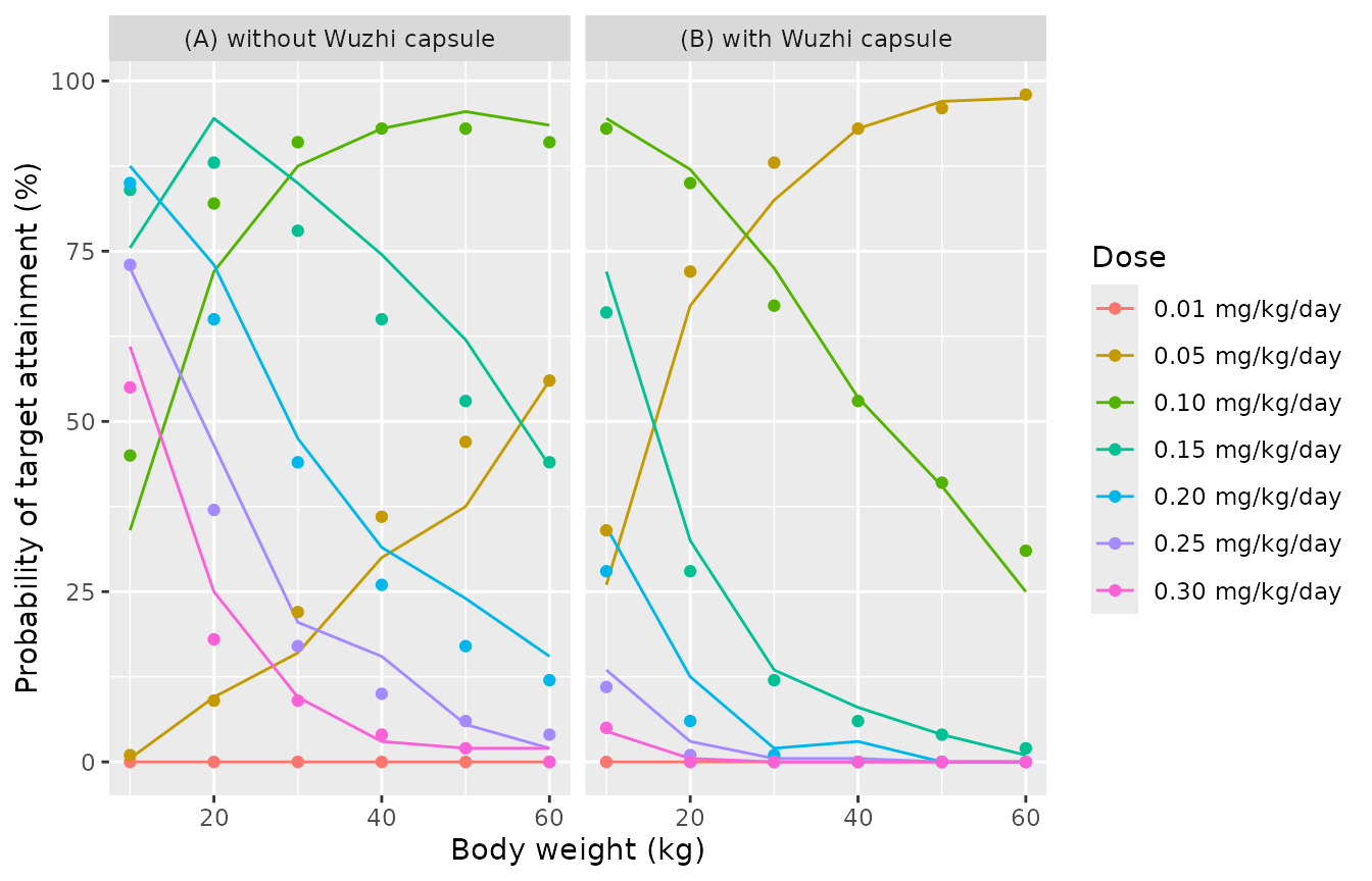
Simulated probability of a 5-15 ng/mL trough (lines) against values digitised from Figure 4 of Chen 2020 (points). Replicates Figure 4 of Chen 2020.
The recommended regimens of Table III follow from these curves: without Wuzhi capsule 0.15 mg/kg/day below 23 kg and 0.10 mg/kg/day above; with Wuzhi capsule 0.10 and 0.05 mg/kg/day respectively.
PKNCA validation
The paper reports no NCA. As a structural check, typical-value
subjects (zeroRe()) at each Figure 4 weight, with and
without Wuzhi capsule, receive 0.10 mg/kg/day split into two doses for 7
days. PKNCA computes the steady-state AUC over the last dosing interval,
which must equal the closed form Dose / (CL/F).
tlast <- tobs - 12
ev_nca <- tidyr::expand_grid(CONMED_WUZHI = 0:1, WT = weights) |>
  mutate(id = row_number())
nca_dose <- ev_nca |>
  tidyr::expand_grid(time = dtimes) |>
  mutate(amt = 0.10 * WT / 2, evid = 1L, cmt = "depot")
nca_obs <- ev_nca |>
  tidyr::expand_grid(time = tlast + c(0, 0.25, 0.5, 1, 1.5, 2, 3, 4, 6, 8, 10, 12)) |>
  mutate(amt = 0, evid = 0L, cmt = "central")
ev_nca_all <- bind_rows(nca_dose, nca_obs) |>
  arrange(id, time, desc(evid)) |>
  mutate(treatment = paste0(WT, " kg, WZ=", CONMED_WUZHI))

sim_nca <- rxode2::rxSolve(mod_typ, events = ev_nca_all, keep = c("WT", "CONMED_WUZHI", "treatment")) |>
  as.data.frame()
#> ℹ omega/sigma items treated as zero: 'etalcl'
#> Warning: multi-subject simulation without without 'omega'

conc <- sim_nca |>
  filter(!is.na(Cc), time >= tlast) |>
  select(id, time, Cc, treatment)
doses <- ev_nca_all |>
  filter(evid == 1, time == tlast) |>
  select(id, time, amt, treatment)

o_conc <- PKNCAconc(conc, Cc ~ time | treatment + id)
o_dose <- PKNCAdose(doses, amt ~ time | treatment + id)
intervals <- data.frame(start = tlast, end = tlast + 12, auclast = TRUE, cmin = TRUE, cmax = TRUE)
nca_res <- pk.nca(PKNCAdata(o_conc, o_dose, intervals = intervals))

nca_wide <- as.data.frame(nca_res) |>
  select(treatment, PPTESTCD, PPORRES) |>
  tidyr::pivot_wider(names_from = PPTESTCD, values_from = PPORRES) |>
  left_join(distinct(ev_nca_all, treatment, WT, CONMED_WUZHI), by = "treatment") |>
  mutate(auc_closed = 1000 * 0.10 * WT / 2 / (15.5 * (WT / 70)^0.75 * (1 - 0.290 * CONMED_WUZHI))) |>
  arrange(CONMED_WUZHI, WT)

nca_wide |>
  select(WT, CONMED_WUZHI, auclast, auc_closed, cmax, cmin) |>
  dplyr::rename(
    "Weight (kg)" = WT, "Wuzhi capsule" = CONMED_WUZHI,
    "AUCtau (PKNCA, ng*h/mL)" = auclast, "Dose/(CL/F) (ng*h/mL)" = auc_closed,
    "Cmax (ng/mL)" = cmax, "Cmin (ng/mL)" = cmin
  ) |>
knitr::kable(digits = 2, caption = "Typical-value steady-state NCA, 0.10 mg/kg/day in two doses.")| Weight (kg) | Wuzhi capsule | AUCtau (PKNCA, ng*h/mL) | Dose/(CL/F) (ng*h/mL) | Cmax (ng/mL) | Cmin (ng/mL) |
|---|---|---|---|---|---|
| 10 | 0 | 138.21 | 138.82 | 21.58 | 4.43 |
| 20 | 0 | 164.48 | 165.09 | 23.59 | 6.24 |
| 30 | 0 | 182.10 | 182.70 | 24.96 | 7.50 |
| 40 | 0 | 195.72 | 196.33 | 26.03 | 8.51 |
| 50 | 0 | 206.98 | 207.59 | 26.91 | 9.35 |
| 60 | 0 | 216.67 | 217.27 | 27.68 | 10.08 |
| 10 | 1 | 194.92 | 195.53 | 25.96 | 8.45 |
| 20 | 1 | 231.92 | 232.52 | 28.89 | 11.25 |
| 30 | 1 | 256.72 | 257.33 | 30.88 | 13.17 |
| 40 | 1 | 275.91 | 276.51 | 32.42 | 14.67 |
| 50 | 1 | 291.77 | 292.38 | 33.70 | 15.92 |
| 60 | 1 | 305.41 | 306.01 | 34.80 | 17.00 |
Assumptions and deviations
-
IIV scale. Table II reports “omega CL/F = 0.172”
without stating whether it is a variance or an SD. Simulating Figure 4
under both readings settles it: with 0.172 as the SD of eta (variance
0.029584) the simulated probabilities follow the published curves
(e.g. 40 kg, 0.10 mg/kg/day, no Wuzhi: about 93% simulated vs 93%
published; 60 kg, 0.05 mg/kg/day with Wuzhi: about 97% vs 98%), whereas
treating 0.172 as the variance (SD 0.415) flattens every curve to
roughly 40-60% (about 56% and 64% at those two points). The SD reading
is used, the same convention the sister paper from this centre (Wang
2019, SOJIA;
Wang_2019b_tacrolimus) resolves to. - Residual error scale and Figure 4. sigma1 = 0.281 is taken as the proportional SD (28.1%), consistent with the omega reading. Figure 4 is reproduced by individual predictions without residual error; adding the proportional error lowers the 40 kg, 0.10 mg/kg/day probability to about 81%, well below the published 93%.
- Sampling time. The paper does not state when the TDM samples were drawn. The fixed ka and the Figure 4 replication (steady-state trough before the next dose) are consistent with trough sampling.
- Figure 4 regimen. “Split into two doses” is read as equal doses every 12 h. The simulation runs 7 days (more than 10 half-lives at every weight) in place of an explicit steady-state solve.
- Digitisation. Figure 3 and Figure 4 values were read off the published figures at the six simulated weights; Excel-style smoothing between those points is ignored. The largest Figure 4 discrepancy (about 8 percentage points at 20 kg without Wuzhi) is at the steepest part of the curves.
- Wuzhi capsule indicator. The paper does not state whether it was time-varying; it is accepted per record. The Wuzhi dose is not reported.
- Fixed ka is inherited from earlier pediatric models and is not identifiable from TDM data.
- The body-weight reference (70 kg) lies above the observed median (47 kg); the typical CL/F of 15.5 L/h is an adult-equivalent value.