Funobactam murine thigh-infection PK (Fratoni 2023)
Source:vignettes/articles/Fratoni_2023_funobactam_mouse.Rmd
Fratoni_2023_funobactam_mouse.RmdModel and source
mod <- rxode2::rxode(readModelDb("Fratoni_2023_funobactam_mouse"))- Article: https://doi.org/10.1093/jac/dkad242
Preclinical (mouse). One-compartment pharmacokinetic model for the beta-lactamase inhibitor funobactam (formerly XNW4107) in the neutropenic murine thigh infection model, with first-order absorption from a subcutaneous depot and first-order elimination (Fratoni 2023). Funobactam was given subcutaneously at 1, 10 and 20 mg/kg together with an imipenem human-simulated regimen in uranyl-nitrate-treated mice (renal impairment induced to slow clearance), and a single best-fit average parameter set was estimated in Phoenix WinNonlin from destructive-sampling mean profiles. Cc is the total plasma concentration that was assayed; Cu is the unbound concentration (mean mouse plasma protein binding 3.53%) that the authors used for every %fT>MIC, %fT>CT, fAUC and fCmax exposure index. The apparent volume is 0.462 L/kg, one tenth of the 4.62 L/kg printed in the Results: only 0.462 L/kg reproduces the authors’ own simulated exposures in Table S1 and Table 2 (see the vignette). No between-subject variability or residual error was reported, so the model has no etas and the residual SD is fixed(0).
Full citation: Fratoni AJ, Berry AV, Liu X, Chen X, Wu Y, Nicolau DP, Abdelraouf K. Imipenem/funobactam (formerly XNW4107) in vivo pharmacodynamics against serine carbapenemase-producing Gram-negative bacteria: a novel modelling approach for time-dependent killing. J Antimicrob Chemother. 2023;78(9):2343-2353. doi:10.1093/jac/dkad242. PK parameters from Results (‘PK studies’); protein binding from Results (‘Ex vivo plasma protein-binding’); simulated exposures used to pin the volume from Supplementary Table S1 and Table 2.
The paper is a pharmacodynamic study of the beta-lactamase inhibitor
funobactam given with a human-simulated imipenem regimen. Its only
fitted time-course model is the one-compartment murine plasma PK model
packaged here; every exposure index the paper analyses
(fAUC0-24, fCmax, %fT>MIC,
%fT>CT) was simulated from that model.
Population
Specific-pathogen-free female ICR mice weighing 20-22 g were rendered neutropenic with cyclophosphamide (150 mg/kg four days and 100 mg/kg one day before inoculation), given uranyl nitrate 5 mg/kg three days before inoculation to reduce renal clearance, and inoculated intramuscularly in one thigh with 0.1 mL of a ~10^7 cfu/mL suspension two hours before treatment (Methods, “Animals” and “Neutropenic murine thigh infection model”). For the PK study, funobactam 1, 10 or 20 mg/kg was given subcutaneously together with the imipenem human-simulated regimen to 36 infected mice per dose (108 in total), sacrificed in groups of six at predefined times for cardiac-puncture plasma (Methods, “Funobactam single-dose studies”). Total funobactam was assayed by LC-MS/MS and the mean profiles were fitted in Phoenix WinNonlin 8.1.
str(mod$population)
#> List of 8
#>  $ species       : chr "mouse (ICR, female, neutropenic thigh infection model)"
#>  $ n_subjects    : num 108
#>  $ n_studies     : num 1
#>  $ weight_range  : chr "20-22 g"
#>  $ sex_female_pct: num 100
#>  $ disease_state : chr "Neutropenic murine thigh infection. Mice were rendered neutropenic with cyclophosphamide (150 mg/kg day -4, 100"| __truncated__
#>  $ dose_range    : chr "funobactam 1, 10 and 20 mg/kg subcutaneously (single dose) with the imipenem human-simulated regimen (8, 2.5, 1"| __truncated__
#>  $ notes         : chr "Methods, 'Funobactam single-dose studies': 36 infected mice per funobactam dose level (108 total), sacrificed i"| __truncated__
Source trace
| Equation / parameter | Value | Source location |
|---|---|---|
lka (ka) |
7.21 1/h | Results, “PK studies”: “first-order absorption rate constant, 7.21 h-1” |
lvc (V/F) |
0.462 L/kg | Results, “PK studies” prints 4.62 L/kg; 0.462 L/kg reproduces Table S1 and Table 2 (see Errata) |
lkel (kel) |
0.41 1/h | Results, “PK studies”: “overall elimination rate constant, 0.41 h-1” |
fu |
0.9647 | Results, “Ex vivo plasma protein-binding”: overall average binding 3.53%; 1 - 0.0353 |
propSd |
fixed(0) | not reported (see Errata) |
d/dt(depot), d/dt(central)
|
n/a | Results, “PK studies”: “PK was best described using a one-compartment model”; subcutaneous dosing with first-order absorption |
Cu <- fu * Cc |
n/a | Methods, “Human-simulated exposure PK studies” and Table 2 / Table S1: all indices use free plasma concentrations |
Virtual cohort
The model has no between-subject variability: each dose level was a
single naive-pooled mean profile from destructively sampled mice. The
replication is therefore deterministic, with one simulated mouse per
regimen. There are no etas, so neither zeroRe() nor
omega = NA is needed (and omega = NA would
error on a model with no random effects).
# Supplementary Table S1 (dose fractionation) and Table 2 (dose ranging).
# Published free exposures over the first 24 h of dosing.
regimens <- tibble::tribble(
  ~treatment,          ~dose, ~tau, ~study,             ~auclast, ~cmax,
  "0.9 mg/kg q6h",     0.9,   6,    "Table S1",          17.8,     1.7,
  "1.8 mg/kg q12h",    1.8,   12,   "Table S1",          18.2,     3.2,
  "3.6 mg/kg q24h",    3.6,   24,   "Table S1",          18.3,     6.3,
  "1.2 mg/kg q4h",     1.2,   4,    "Table S1",          35.0,     2.6,
  "1.8 mg/kg q6h",     1.8,   6,    "Table S1",          35.7,     3.5,
  "3.6 mg/kg q12h",    3.6,   12,   "Table S1",          36.4,     6.4,
  "7.2 mg/kg q24h",    7.2,   24,   "Table S1",          36.6,     12.6,
  "3.6 mg/kg q6h",     3.6,   6,    "Table 2 (interp.)", 71.36,    6.95,
  "7.2 mg/kg q6h",     7.2,   6,    "Table 2 (obs.)",    142.71,   13.90,
  "14.4 mg/kg q6h",    14.4,  6,    "Table 2 (obs.)",    363.70,   36.15
)
stopifnot(!anyDuplicated(regimens$treatment))

make_events <- function(dose, tau, id, treatment) {
  addl <- 24 / tau - 1
  # A once-daily regimen is a single dose within the 24 h window; rxode2
  # resets a non-zero `ii` with `addl = 0` and warns, so pass `ii = 0` there.
  ii <- if (addl > 0) tau else 0
  rxode2::et(amt = dose, ii = ii, addl = addl, cmt = "depot") |>
    rxode2::et(seq(0, 24, by = 0.01), cmt = "central") |>
    as.data.frame() |>
    dplyr::mutate(id = id, treatment = treatment)
}
events <- dplyr::bind_rows(lapply(seq_len(nrow(regimens)), function(i) {
  make_events(regimens$dose[i], regimens$tau[i], i, regimens$treatment[i])
}))Replicate published figures
Figure 1: free plasma concentration over the first dosing interval
Figure 1 overlays the free funobactam profile of each dose-ranging regimen (0.9, 1.8, 3.6, 7.2 and 14.4 mg/kg q6h) over one 6 h interval. The lines below are the packaged typical-value model; the paper’s 14.4 mg/kg line was drawn from that dose’s own confirmatory PK study, which ran about 25% above dose proportionality (see the NCA comparison below).
sim |>
  dplyr::filter(grepl("q6h$", treatment), time <= 6) |>
  dplyr::mutate(treatment = factor(
    treatment,
    levels = c("14.4 mg/kg q6h", "7.2 mg/kg q6h", "3.6 mg/kg q6h",
               "1.8 mg/kg q6h", "0.9 mg/kg q6h")
  )) |>
  ggplot(aes(time, Cu, colour = treatment)) +
  geom_line(linewidth = 0.8) +
  scale_y_log10(limits = c(0.01, 100)) +
  labs(x = "Time (h)", y = "Free plasma funobactam (mg/L)", colour = "Regimen",
       title = "Replicates Figure 1 of Fratoni 2023",
       caption = "Typical-value model; observed means are not reproduced.") +
  theme_bw()
#> Warning in scale_y_log10(limits = c(0.01, 100)): log-10 transformation
#> introduced infinite values.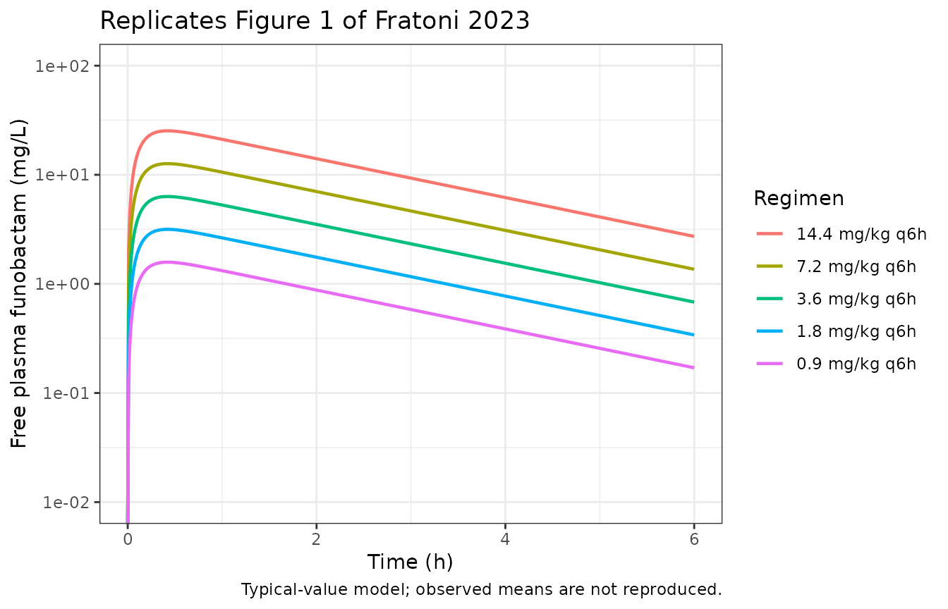
Supplementary Table S1: %fT>MIC of the dose-fractionation regimens
Table S1 was generated by the authors by simulating each
dose-fractionation regimen “using parameters from single dose PK
studies”, so it is a direct check of the packaged parameters.
%fT>MIC is the percentage of the first 24 h with free
concentration above each MIC.
mics <- c(0.25, 0.5, 1, 2, 4, 8)
published_ft <- tibble::tribble(
  ~treatment,       ~`0.25`, ~`0.5`, ~`1`, ~`2`, ~`4`, ~`8`,
  "0.9 mg/kg q6h",  86,      57,     29,   0,    0,    0,
  "1.8 mg/kg q12h", 56,      42,     28,   13,   0,    0,
  "3.6 mg/kg q24h", 35,      28,     21,   14,   6,    0,
  "1.2 mg/kg q4h",  100,     100,    69,   24,   0,    0,
  "1.8 mg/kg q6h",  100,     86,     57,   29,   6,    0,
  "3.6 mg/kg q12h", 70,      56,     42,   28,   13,   0,
  "7.2 mg/kg q24h", 42,      35,     28,   21,   14,   6
) |>
  tidyr::pivot_longer(-treatment, names_to = "MIC", values_to = "published") |>
  dplyr::mutate(MIC = as.numeric(MIC))

sim_ft <- sim |>
  dplyr::filter(time < 24) |>
  tidyr::crossing(MIC = mics) |>
  dplyr::group_by(treatment, MIC) |>
  dplyr::summarise(simulated = 100 * mean(Cu > MIC), .groups = "drop")

ft_cmp <- published_ft |>
  dplyr::inner_join(sim_ft, by = c("treatment", "MIC"))
stopifnot(nrow(ft_cmp) == nrow(published_ft))

ft_cmp |>
  dplyr::mutate(simulated = round(simulated, 1),
                diff = round(simulated - published, 1)) |>
  dplyr::rename("Regimen" = treatment, "MIC (mg/L)" = MIC,
                "Published %fT>MIC" = published,
                "Simulated %fT>MIC" = simulated,
                "Difference (points)" = diff) |>
knitr::kable(caption = "Supplementary Table S1 %fT>MIC replication.")| Regimen | MIC (mg/L) | Published %fT>MIC | Simulated %fT>MIC | Difference (points) |
|---|---|---|---|---|
| 0.9 mg/kg q6h | 0.25 | 86 | 86.9 | 0.9 |
| 0.9 mg/kg q6h | 0.50 | 57 | 58.3 | 1.3 |
| 0.9 mg/kg q6h | 1.00 | 29 | 29.2 | 0.2 |
| 0.9 mg/kg q6h | 2.00 | 0 | 0.0 | 0.0 |
| 0.9 mg/kg q6h | 4.00 | 0 | 0.0 | 0.0 |
| 0.9 mg/kg q6h | 8.00 | 0 | 0.0 | 0.0 |
| 1.8 mg/kg q12h | 0.25 | 56 | 56.3 | 0.3 |
| 1.8 mg/kg q12h | 0.50 | 42 | 42.2 | 0.2 |
| 1.8 mg/kg q12h | 1.00 | 28 | 27.8 | -0.2 |
| 1.8 mg/kg q12h | 2.00 | 13 | 13.2 | 0.2 |
| 1.8 mg/kg q12h | 4.00 | 0 | 0.0 | 0.0 |
| 1.8 mg/kg q12h | 8.00 | 0 | 0.0 | 0.0 |
| 3.6 mg/kg q24h | 0.25 | 35 | 35.2 | 0.2 |
| 3.6 mg/kg q24h | 0.50 | 28 | 28.1 | 0.1 |
| 3.6 mg/kg q24h | 1.00 | 21 | 21.0 | 0.0 |
| 3.6 mg/kg q24h | 2.00 | 14 | 13.9 | -0.1 |
| 3.6 mg/kg q24h | 4.00 | 6 | 6.6 | 0.6 |
| 3.6 mg/kg q24h | 8.00 | 0 | 0.0 | 0.0 |
| 1.2 mg/kg q4h | 0.25 | 100 | 99.9 | -0.1 |
| 1.2 mg/kg q4h | 0.50 | 100 | 99.8 | -0.2 |
| 1.2 mg/kg q4h | 1.00 | 69 | 69.2 | 0.2 |
| 1.2 mg/kg q4h | 2.00 | 24 | 24.0 | 0.0 |
| 1.2 mg/kg q4h | 4.00 | 0 | 0.0 | 0.0 |
| 1.2 mg/kg q4h | 8.00 | 0 | 0.0 | 0.0 |
| 1.8 mg/kg q6h | 0.25 | 100 | 100.0 | 0.0 |
| 1.8 mg/kg q6h | 0.50 | 86 | 86.9 | 0.9 |
| 1.8 mg/kg q6h | 1.00 | 57 | 58.3 | 1.3 |
| 1.8 mg/kg q6h | 2.00 | 29 | 29.2 | 0.2 |
| 1.8 mg/kg q6h | 4.00 | 6 | 0.0 | -6.0 |
| 1.8 mg/kg q6h | 8.00 | 0 | 0.0 | 0.0 |
| 3.6 mg/kg q12h | 0.25 | 70 | 70.4 | 0.4 |
| 3.6 mg/kg q12h | 0.50 | 56 | 56.3 | 0.3 |
| 3.6 mg/kg q12h | 1.00 | 42 | 42.2 | 0.2 |
| 3.6 mg/kg q12h | 2.00 | 28 | 27.8 | -0.2 |
| 3.6 mg/kg q12h | 4.00 | 13 | 13.2 | 0.2 |
| 3.6 mg/kg q12h | 8.00 | 0 | 0.0 | 0.0 |
| 7.2 mg/kg q24h | 0.25 | 42 | 42.2 | 0.2 |
| 7.2 mg/kg q24h | 0.50 | 35 | 35.2 | 0.2 |
| 7.2 mg/kg q24h | 1.00 | 28 | 28.1 | 0.1 |
| 7.2 mg/kg q24h | 2.00 | 21 | 21.0 | 0.0 |
| 7.2 mg/kg q24h | 4.00 | 14 | 13.9 | -0.1 |
| 7.2 mg/kg q24h | 8.00 | 6 | 6.6 | 0.6 |
# Same parameters on both sides: the only difference is the authors' rounding
# and time grid, so a tight bound is appropriate. The 1.8 mg/kg q6h cell at
# MIC 4 is excluded: Table S1 prints 6%, but the same row's fCmax is 3.5 mg/L
# (below 4) and Table 2 prints 0% for the identical regimen.
slip <- ft_cmp$treatment == "1.8 mg/kg q6h" & ft_cmp$MIC == 4
stopifnot(sum(slip) == 1, ft_cmp$simulated[slip] == 0)
stopifnot(max(abs(ft_cmp$simulated[!slip] - ft_cmp$published[!slip])) < 2.5)
41 of the 42 cells agree within 1.3 percentage points. The remaining
cell, 1.8 mg/kg q6h at an MIC of 4 mg/L, is printed as 6% in Table S1.
That is inconsistent with the paper itself: the row’s own
fCmax is 3.5 mg/L, so the free concentration never reaches
4 mg/L, and Table 2 gives 0% for the same regimen at the same MIC. The
simulated 0% agrees with Table 2.
PKNCA validation
nca_conc <- sim |>
  dplyr::filter(!is.na(Cu)) |>
  dplyr::select(id, time, Cu, treatment)
# Guarantee a time-zero row (pre-dose free concentration is zero).
nca_conc <- dplyr::bind_rows(
  nca_conc,
  nca_conc |> dplyr::distinct(id, treatment) |> dplyr::mutate(time = 0, Cu = 0)
) |>
  dplyr::distinct(id, treatment, time, .keep_all = TRUE) |>
  dplyr::arrange(id, time)

nca_dose <- dplyr::bind_rows(lapply(seq_len(nrow(regimens)), function(i) {
  data.frame(id = i, treatment = regimens$treatment[i],
             amt = regimens$dose[i],
             time = seq(0, 24 - regimens$tau[i], by = regimens$tau[i]))
}))

conc_obj <- PKNCA::PKNCAconc(nca_conc, Cu ~ time | treatment + id,
                             concu = "mg/L", timeu = "h")
dose_obj <- PKNCA::PKNCAdose(nca_dose, amt ~ time | treatment + id,
                             doseu = "mg/kg")
intervals <- data.frame(start = 0, end = 24, cmax = TRUE, tmax = TRUE,
                        auclast = TRUE)
nca_res <- PKNCA::pk.nca(PKNCA::PKNCAdata(conc_obj, dose_obj,
                                          intervals = intervals))
Comparison against published NCA
Table S1 rows and the Table 2 row marked “interp.” were computed by the authors from the single-dose model; the Table 2 rows marked “obs.” are from separate confirmatory PK studies at those doses.
cmp <- nlmixr2lib::ncaComparisonTable(
  simulated = nca_res,
  reference = regimens |> dplyr::select(treatment, auclast, cmax),
  by = "treatment",
  units = c(auclast = "mg*h/L", cmax = "mg/L"),
  tolerance_pct = 20
)
knitr::kable(cmp, caption = paste(
  "Simulated vs published free funobactam fAUC0-24 and fCmax.",
  "* differs by >20%."
))| NCA parameter | treatment | Reference | Simulated | % diff |
|---|---|---|---|---|
| Cmax (mg/L) | 0.9 mg/kg q6h | 1.7 | 1.74 | +2.2% |
| Cmax (mg/L) | 1.8 mg/kg q12h | 3.2 | 3.19 | -0.4% |
| Cmax (mg/L) | 3.6 mg/kg q24h | 6.3 | 6.32 | +0.4% |
| Cmax (mg/L) | 1.2 mg/kg q4h | 2.6 | 2.65 | +1.9% |
| Cmax (mg/L) | 1.8 mg/kg q6h | 3.5 | 3.48 | -0.7% |
| Cmax (mg/L) | 3.6 mg/kg q12h | 6.4 | 6.37 | -0.4% |
| Cmax (mg/L) | 7.2 mg/kg q24h | 12.6 | 12.6 | +0.4% |
| Cmax (mg/L) | 3.6 mg/kg q6h | 6.95 | 6.95 | +0.0% |
| Cmax (mg/L) | 7.2 mg/kg q6h | 13.9 | 13.9 | +0.0% |
| Cmax (mg/L) | 14.4 mg/kg q6h | 36.2 | 27.8 | -23.1%* |
| AUClast (mg*h/L) | 0.9 mg/kg q6h | 17.8 | 17.9 | +0.4% |
| AUClast (mg*h/L) | 1.8 mg/kg q12h | 18.2 | 18.3 | +0.3% |
| AUClast (mg*h/L) | 3.6 mg/kg q24h | 18.3 | 18.3 | +0.2% |
| AUClast (mg*h/L) | 1.2 mg/kg q4h | 35 | 35.1 | +0.3% |
| AUClast (mg*h/L) | 1.8 mg/kg q6h | 35.7 | 35.8 | +0.2% |
| AUClast (mg*h/L) | 3.6 mg/kg q12h | 36.4 | 36.5 | +0.3% |
| AUClast (mg*h/L) | 7.2 mg/kg q24h | 36.6 | 36.7 | +0.2% |
| AUClast (mg*h/L) | 3.6 mg/kg q6h | 71.4 | 71.5 | +0.2% |
| AUClast (mg*h/L) | 7.2 mg/kg q6h | 143 | 143 | +0.2% |
| AUClast (mg*h/L) | 14.4 mg/kg q6h | 364 | 286 | -21.3%* |
attr(cmp, "footnote")
#> [1] "* differs from reference by more than ±20%."

nca_wide <- as.data.frame(nca_res$result) |>
  dplyr::filter(PPTESTCD %in% c("auclast", "cmax")) |>
  dplyr::select(treatment, PPTESTCD, PPORRES) |>
  tidyr::pivot_wider(names_from = PPTESTCD, values_from = PPORRES) |>
  dplyr::inner_join(
    regimens |> dplyr::select(treatment, study, pub_auc = auclast,
                              pub_cmax = cmax),
    by = "treatment"
  )
stopifnot(nrow(nca_wide) == nrow(regimens))

# Model-derived rows (Table S1 and the interpolated Table 2 row) must match to
# the authors' rounding.
model_rows <- nca_wide |> dplyr::filter(study != "Table 2 (obs.)")
stopifnot(
  max(abs(model_rows$auclast / model_rows$pub_auc - 1)) < 0.02,
  max(abs(model_rows$cmax - model_rows$pub_cmax)) < 0.06
)
All model-derived rows agree with the published values to their printed rounding. The 7.2 mg/kg q6h confirmatory study also agrees within 1%. The 14.4 mg/kg q6h confirmatory study is about 21-23% above the model. The paper does not discuss the excess; it used that study’s observed exposures directly rather than the model, so the starred row reflects the confirmatory data and not the extraction.
The printed volume
The Results print the apparent volume as 4.62 L/kg. Simulating the same regimens with that value shows it cannot be what the authors used:
sim_printed <- rxode2::rxSolve(mod, events, keep = "treatment",
                               params = c(lvc = log(4.62)),
                               returnType = "data.frame")
#> Warning: multi-subject simulation without without 'omega'
printed_auc <- sim_printed |>
  dplyr::filter(time <= 24) |>
  dplyr::group_by(treatment) |>
  dplyr::summarise(auc_printed = sum(diff(time) *
    (head(Cu, -1) + tail(Cu, -1)) / 2), .groups = "drop")

nca_wide |>
  dplyr::inner_join(printed_auc, by = "treatment") |>
  dplyr::filter(study == "Table S1") |>
  dplyr::transmute(treatment, pub_auc,
                   auc_0462 = round(auclast, 2),
                   auc_462 = round(auc_printed, 2)) |>
  dplyr::rename("Regimen" = treatment,
                "Table S1 fAUC0-24" = pub_auc,
                "Simulated, V/F = 0.462 L/kg" = auc_0462,
                "Simulated, V/F = 4.62 L/kg" = auc_462) |>
knitr::kable(caption = "Table S1 fAUC0-24 (mg*h/L) under both readings.")| Regimen | Table S1 fAUC0-24 | Simulated, V/F = 0.462 L/kg | Simulated, V/F = 4.62 L/kg |
|---|---|---|---|
| 0.9 mg/kg q6h | 17.8 | 17.88 | 1.79 |
| 1.2 mg/kg q4h | 35.0 | 35.11 | 3.51 |
| 1.8 mg/kg q12h | 18.2 | 18.26 | 1.83 |
| 1.8 mg/kg q6h | 35.7 | 35.76 | 3.58 |
| 3.6 mg/kg q12h | 36.4 | 36.53 | 3.65 |
| 3.6 mg/kg q24h | 18.3 | 18.33 | 1.83 |
| 7.2 mg/kg q24h | 36.6 | 36.67 | 3.67 |
Assumptions and deviations
-
Volume of distribution. The Results print
V = 4.62 L/kg. The packaged value is 0.462 L/kg. The authors’ own simulated exposures (Supplementary Table S1, seven regimens, each withfAUC0-24,fCmaxand six%fT>MICvalues), the interpolated Table 2 rows, the 7.2 mg/kg q6h confirmatory study and the Figure 1 curves are all reproduced to their rounding with 0.462 L/kg, and are all ten-fold higher than 4.62 L/kg gives. SinceAUC = dose / (V * kel), the gap could otherwise only come fromkel, but a ten-fold smallerkelwould also change theCmaxand the%fT>MICdurations, which 0.462 L/kg reproduces. The printed value is therefore treated as a decimal-place slip. -
Table S1 cell. Supplementary Table S1 prints
%fT>MIC = 6%for 1.8 mg/kg q6h at an MIC of 4 mg/L. The same row’sfCmax(3.5 mg/L) and Table 2 (0% for the identical regimen) both contradict it, so it is treated as a typesetting slip and excluded from the numerical check. -
Free fraction.
fu = 0.9647is one minus the overall mean protein binding of 3.53%. The authors state binding was low and not concentration-dependent over 1-20 mg/kg;fuis held fixed. -
No variability. The PK study was destructive
sampling with six mice per time point, fitted to mean profiles, so no
between-subject variability exists to report. The paper reports no
residual error model either;
propSdisfixed(0)and the model is suitable for typical-value simulation only. -
Bioavailability. Dosing was subcutaneous only, so
bioavailability is absorbed into the apparent volume
V/F. - Imipenem not modelled. The imipenem human-simulated regimen was designed from murine imipenem PK parameters published earlier by the same group and not reported in this paper. The paper shows funobactam did not alter imipenem exposure (Figure 2), so the funobactam model stands alone.
-
Exposure-response not extracted. The paper’s
sigmoid Emax fits relate a 24 h summary index (
fAUC/MIC,fCmax/MIC,%fT>MIC,%fT>CT,(%fT>CT)/MIC) to the 24 h change in log10 cfu/thigh. They have no time course, and the paper reports only the derived stasis / 1-log / 2-log targets andR^2(Tables 4, 5 and S2), notE0,Emax,EC50or the Hill coefficient. TheCuoutput is what a user needs to compute any of these indices for a new regimen.