Sipoglitazar (Stringer 2014)
Source:vignettes/articles/Stringer_2014_sipoglitazar.Rmd
Stringer_2014_sipoglitazar.RmdModel and source
- Citation: Stringer F, DeJongh J, Scott G, Danhof M. A Model-Based Approach to Analyze the Influence of UGT2B15 Polymorphism Driven Pharmacokinetic Differences on the Pharmacodynamic Response of the PPAR Agonist Sipoglitazar. J Clin Pharmacol. 2014;54(4):453-461. doi:10.1002/jcph.227. Per-genotype sipoglitazar clearance values reproduced in Table 1 originate from the companion population PK analysis, Stringer F, Ploeger BA, DeJongh J, et al. J Clin Pharmacol. 2013;53(3):256-263.
- Description: Simultaneous, cascading indirect-response PK/PD model for fasting plasma glucose (FPG) and glycosylated hemoglobin (HbA1c) in 780 drug-naive Type 2 diabetes mellitus patients treated for 13 weeks with the PPAR alpha/delta/gamma agonist sipoglitazar, rosiglitazone 8 mg once daily, or placebo (Stringer 2014). FPG is a zero-order production / first-order loss turnover pool (KinG, KoutG); HbA1c is a secondary cascade driven by a power function of FPG (FPG^gamma, gamma = 0.71) with first-order production and degradation (KinH, KoutH). The sipoglitazar effect stimulates KoutG through an Emax function of steady-state exposure, AUC0-24h = total daily dose / CL, where CL is fixed per UGT2B15 genotype (5.04, 3.35 and 1.53 L/h for UGT2B151/1, 1/2 and 2/2 respectively; Table 1) so that genotype-driven exposure differences propagate into the glycemic response. Rosiglitazone enters as a fixed 28% stimulatory step on KoutG (ROTE). Two study-conduct ‘lifestyle’ effects are carried: LEFPG, a mean-zero additive random effect on KinG capturing per-subject diet / exercise improvement or loss of glycemic control, and LEHB, a step inhibition of KinH that is larger in the placebo arm (3.7%) than in the sipoglitazar arms (2.0%) and absent on rosiglitazone. This is a PD-only model: no drug is dosed through the event table – exposure is supplied through the DOSE_SIPOGLITAZAR_MGD and UGT2B15 genotype covariates. No demographic covariate (age, sex, weight, duration of disease) was retained.
- Article: https://doi.org/10.1002/jcph.227
Sipoglitazar is an oral PPAR alpha/delta/gamma agonist that is
cleared by UDP-glucuronosyltransferase 2B15. The UGT2B15*2
allele reduces glucuronidation, so UGT2B15*2/*2 subjects
clear the drug about 3.3-fold more slowly than UGT2B15*1/*1
subjects and reach correspondingly higher exposure. The question this
paper asks is whether that pharmacokinetic difference is large enough to
matter clinically – i.e. whether it propagates into the glycemic
response – and whether genotype-guided dose selection can equalise
it.
The model is pharmacodynamic only. No drug is dosed
through the event table and there is no plasma concentration state:
exposure enters as a steady-state AUC0-24h computed from
the subject’s total daily dose and genotype-specific clearance.
Consequently there is nothing for a non-compartmental analysis to
integrate, and this vignette uses the turnover-model validation strategy
(steady-state identities, closed-form checks, perturbation recovery, and
replication of the paper’s own published simulations) rather than a
PKNCA section.
# Build the two model objects from INDEPENDENT rxode() calls. rxode2's
# zeroRe() modifies the object it is handed, so `mod_typ <- zeroRe(mod_iiv)`
# would silently zero the omega of `mod_iiv` as well and every "with IIV"
# simulation below would quietly run at the typical value.
mod_iiv <- rxode2::rxode(readModelDb("Stringer_2014_sipoglitazar"))
#> ℹ parameter labels from comments will be replaced by 'label()'
#> Warning: some etas defaulted to non-mu referenced, possible parsing error: etalrbase_hba1c
#> as a work-around try putting the mu-referenced expression on a simple line
mod_typ <- rxode2::zeroRe(rxode2::rxode(readModelDb("Stringer_2014_sipoglitazar")))
#> ℹ parameter labels from comments will be replaced by 'label()'
#> Warning: some etas defaulted to non-mu referenced, possible parsing error: etalrbase_hba1c
#> as a work-around try putting the mu-referenced expression on a simple line
#> Warning: some etas defaulted to non-mu referenced, possible parsing error: etalrbase_hba1c
#> as a work-around try putting the mu-referenced expression on a simple line
Population
Two 13-week Phase II randomized, double-blind trials in 780 drug-naive adults with type 2 diabetes mellitus were pooled (sipoglitazar n = 572, rosiglitazone n = 72, placebo n = 136). Entry required a diagnosis of type 2 diabetes with no prior anti-diabetic medication, a screening HbA1c above 7.0% and below 10.0%, and age above 35 and below 75 years.
Baseline characteristics (supplement Table S1): age median 56 years
(range 34-75); 388 male / 392 female; body weight median 88.8 kg (range
55-160); duration of disease median 1.0 year (range 0-30.9); FPG
baseline median 9.3 mmol/L (range 2.9-20.8); HbA1c baseline median 7.9%
(range 6.9-9.9). UGT2B15 genotype was *1/*1 :
*1/*2 : *2/*2 = 149 : 357 : 194 among the 700
genotyped subjects (21% : 51% : 28%); genotype was not collected in the
remaining 80 subjects (10%), who were carried with a population-average
clearance.
FPG and HbA1c were sampled at -1, 0, 2, 4, 6, 8, 10 and 12 weeks. All subjects received dietary advice for the whole trial, which is what the model’s LEFPG and LEHB “lifestyle effect” parameters absorb.
The same information is available programmatically via
readModelDb("Stringer_2014_sipoglitazar")()$population.
Source trace
The per-parameter origin is recorded as an in-file comment next to
each ini() entry in
inst/modeldb/specificDrugs/Stringer_2014_sipoglitazar.R.
The tables below collect them in one place for review.
Equations
| Model element | Source location |
|---|---|
DEF = Emax * AUC / (AUC50 + AUC) |
Equation (1), p. 454 |
LEHB_active = LEHB_placebo - LEHB_factor |
Equation (2), p. 455 |
dFPG/dt = KinG * (1 +/- LEFPG) - KoutG * (1 + DEF + ROTE) * FPG |
Equation (3), p. 455 (the paper really does typeset a plus-minus sign here; see Assumptions) |
dHbA1c/dt = KinH * (1 - LEHB) * FPG^gamma - KoutH * HbA1c |
Equation (4), p. 455 |
AUC = total daily dose / CL at steady state |
Methods “Population Data Analysis”, p. 454 |
KinG = KoutG * BSL_FPG (baseline pinning) |
Implied by the indirect-response parameterisation; KinG
is not tabulated |
KinH = KoutH * BSL_HbA1c / BSL_FPG^gamma (baseline
pinning) |
Implied by the indirect-response parameterisation; KinH
is not tabulated |
Box-Cox eta transform
(exp(lambda * eta) - 1) / lambda
|
Methods “Intra-Individual Variability”, citing Petersson 2009 (reference 18) |
Parameters
| Parameter (file) | Paper symbol | Value | Source location |
|---|---|---|---|
lrbase_fpg |
BSL FPG | 9.41 mmol/L | Table 2 |
lrbase_fpg_bid32 |
BSL FPG (32 mg BID) | 9.02 mmol/L | Table 2, footnote a |
lkout_fpg |
KoutG | 0.027 1/day | Table 2 |
lrbase_hba1c |
BSL HbA1c | 7.96 % | Table 2 |
lkout_hba1c |
KoutH | 0.031 1/day | Table 2 |
lgamma |
Gamma (printed as lambda in Eq. 4) | 0.71 | Table 2 |
lemax |
Emax | 48.7 % -> 0.487 fraction | Table 2 |
lauc50 |
AUC50 | 1.15 mg*day/L | Table 2 |
e_rosi_kout_fpg |
ROTE | 0.28 | Table 2 |
e_lifestyle_kin_fpg |
LEFPG | 0 (fixed) | Table 2, footnote b |
e_placebo_kin_hba1c |
LEHB placebo | 0.037 | Table 2 |
e_active_kin_hba1c |
LEHB factor | 0.017 | Table 2, footnote c / Eq. (2) |
boxcox_rbase_hba1c |
Box-Cox | 2.39 | Table 2 |
etalrbase_fpg |
omega^2 BSL FPG | 0.05 | Table 2 |
etalrbase_hba1c |
omega^2 BSL HbA1c | 0.01 | Table 2 |
etae_lifestyle_kin_fpg |
omega^2 LEFPG | 0.04 | Table 2 |
etae_placebo_kin_hba1c |
omega^2 LEHB | 0.01 | Table 2 |
propSd_glucose |
Residual error FPG | 10.6 % -> 0.106 | Table 2 |
propSd_hba1c |
Residual error HbA1c | 2.0 % -> 0.020 | Table 2 |
lcl_ugt2b15_s1s1 |
CL, UGT2B15*1/*1
|
5.04 L/h (fixed) | Table 1 |
lcl_ugt2b15_s1s2 |
CL, UGT2B15*1/*2
|
3.35 L/h (fixed) | Table 1 |
lcl_ugt2b15_s2s2 |
CL, UGT2B15*2/*2
|
1.53 L/h (fixed) | Table 1 |
lcl_ugt2b15_missing |
population-average CL | 3.21 L/h (derived, see Errata) | Not printed; derived from Table 1 + Table S1 |
Dimensional analysis
Time is days throughout, because KoutG
and KoutH are reported in days^-1 and
AUC50 in mg*day/L. Both ODE states are carried
on the measured scale (a concentration and a percentage), not as
amounts, which is the standard indirect-response parameterisation.
| Term | Units | Product |
|---|---|---|
KinG = KoutG * BSL_FPG |
(1/day) * (mmol/L) |
mmol/(L*day) |
KoutG * (1 + DEF + ROTE) * FPG |
(1/day) * (unitless) * (mmol/L) |
mmol/(L*day) |
AUC = dose / (CL * 24) |
mg / ((L/h) * (h/day)) |
mg*day/L, matching AUC50 |
DEF = Emax * AUC / (AUC50 + AUC) |
(unitless) * (mg*day/L)/(mg*day/L) |
unitless |
KinH = KoutH * BSL_HbA1c / BSL_FPG^gamma |
(1/day) * % / (mmol/L)^0.71 |
% * (L/mmol)^0.71 / day |
KinH * (1 - LEHB) * FPG^gamma |
% * (L/mmol)^0.71/day * (mmol/L)^0.71 |
%/day |
KoutH * HbA1c |
(1/day) * % |
%/day |
Both ODE right-hand sides reduce to [state]/day, and the
mmol/L raised to the fractional power gamma
cancels exactly between KinH and the FPG^gamma
driver, so the fractional-power term introduces no residual unit. The
one non-obvious conversion is the * 24 that turns the Table
1 clearances (L/h) into L/day; without it, AUC would be
24-fold too large and every drug effect would saturate.
Structural checks
Placebo FPG holds exactly at baseline
The paper states that “the FPG data in the placebo group on average
showed no change over time” – LEFPG has a population value of exactly
zero. With the random effects zeroed, the placebo FPG trajectory must
therefore be a flat line at 9.41 mmol/L to solver precision. This check
also confirms that zeroRe() actually took effect (any
leaked IIV would move the trajectory).
ev_placebo <- data.frame(
  id = 1L, time = seq(0, 395, by = 5), amt = NA_real_, evid = 0L,
  cmt = "glucose", dvid = 1L,
  TRT = 0, DOSE_SIPOGLITAZAR_MGD = 0,
  UGT2B15_STAR2_HET = 0, UGT2B15_STAR2_HOM = 0, UGT2B15_MISSING = 1
)
s_placebo <- rxode2::rxSolve(mod_typ, ev_placebo, useLinCmt = FALSE) |>
  as.data.frame()
#> ℹ omega/sigma items treated as zero: 'etalrbase_fpg', 'etalrbase_hba1c', 'etae_lifestyle_kin_fpg', 'etae_placebo_kin_hba1c'

stopifnot(max(abs(s_placebo$glucose - 9.41)) < 1e-6)
Placebo HbA1c, by contrast, must decline: LEHB inhibits
KinH by 3.7% in the placebo arm while FPG stays at its
baseline, so the closed-form steady state is
BSL_HbA1c * (1 - LEHB_placebo) exactly.
Closed-form steady state across a dose / genotype ladder
Setting both derivatives to zero gives
FPG_ss   = BSL_FPG / (1 + DEF + ROTE)
HbA1c_ss = BSL_HbA1c * (1 - LEHB) * (FPG_ss / BSL_FPG)^gamma
Because both sides of this comparison use the same parameter draw, the only difference is numerical integration error, so a tight bound is the correct assertion here.
genotypes <- tibble::tibble(
  genotype = c("*1/*1", "*1/*2", "*2/*2"),
  cl_lh    = c(5.04, 3.35, 1.53),
  UGT2B15_STAR2_HET = c(0, 1, 0),
  UGT2B15_STAR2_HOM = c(0, 0, 1)
)

ladder <- tidyr::crossing(genotypes, dose_mgd = c(8, 16, 32, 64, 96)) |>
  dplyr::mutate(
    id = dplyr::row_number(),
    TRT = 1, DOSE_SIPOGLITAZAR_MGD = dose_mgd, UGT2B15_MISSING = 0,
    auc  = dose_mgd / (cl_lh * 24),
    def  = 0.487 * auc / (1.15 + auc),
    lehb = 0.037 - 0.017,
    fpg_cf   = 9.41 / (1 + def),
    hba1c_cf = 7.96 * (1 - lehb) * (fpg_cf / 9.41)^0.71
  )

ev_ladder <- ladder |>
  dplyr::select(id, TRT, DOSE_SIPOGLITAZAR_MGD,
                UGT2B15_STAR2_HET, UGT2B15_STAR2_HOM, UGT2B15_MISSING) |>
  tidyr::crossing(time = c(0, 2000)) |>
  dplyr::mutate(amt = NA_real_, evid = 0L, cmt = "glucose", dvid = 1L)

ss <- rxode2::rxSolve(mod_typ, ev_ladder, useLinCmt = FALSE) |>
  as.data.frame() |>
  dplyr::filter(time == 2000) |>
  dplyr::select(id, fpg_sim = glucose, hba1c_sim = hba1c) |>
  dplyr::left_join(dplyr::select(ladder, id, genotype, dose_mgd, fpg_cf, hba1c_cf),
                   by = "id") |>
  dplyr::mutate(
    fpg_relerr   = abs(fpg_sim   - fpg_cf)   / fpg_cf,
    hba1c_relerr = abs(hba1c_sim - hba1c_cf) / hba1c_cf
  )
#> ℹ omega/sigma items treated as zero: 'etalrbase_fpg', 'etalrbase_hba1c', 'etae_lifestyle_kin_fpg', 'etae_placebo_kin_hba1c'
#> Warning: multi-subject simulation without without 'omega'

stopifnot(max(ss$fpg_relerr) < 1e-5, max(ss$hba1c_relerr) < 1e-5)

ss |>
  dplyr::transmute(
    Genotype = genotype, `Dose (mg/day)` = dose_mgd,
    `FPG closed form` = round(fpg_cf, 3), `FPG solved` = round(fpg_sim, 3),
    `HbA1c closed form` = round(hba1c_cf, 3), `HbA1c solved` = round(hba1c_sim, 3)
  ) |>
knitr::kable(caption = "Solved steady state against the closed form implied by Equations (3) and (4).")| Genotype | Dose (mg/day) | FPG closed form | FPG solved | HbA1c closed form | HbA1c solved |
|---|---|---|---|---|---|
| 1/1 | 8 | 9.167 | 9.167 | 7.657 | 7.657 |
| 1/1 | 16 | 8.960 | 8.960 | 7.534 | 7.534 |
| 1/1 | 32 | 8.624 | 8.624 | 7.333 | 7.333 |
| 1/1 | 64 | 8.158 | 8.158 | 7.049 | 7.049 |
| 1/1 | 96 | 7.849 | 7.849 | 6.858 | 6.858 |
| 1/2 | 8 | 9.059 | 9.059 | 7.593 | 7.593 |
| 1/2 | 16 | 8.779 | 8.779 | 7.426 | 7.426 |
| 1/2 | 32 | 8.363 | 8.363 | 7.174 | 7.174 |
| 1/2 | 64 | 7.847 | 7.847 | 6.857 | 6.857 |
| 1/2 | 96 | 7.540 | 7.540 | 6.665 | 6.665 |
| 2/2 | 8 | 8.733 | 8.733 | 7.398 | 7.398 |
| 2/2 | 16 | 8.299 | 8.299 | 7.135 | 7.135 |
| 2/2 | 32 | 7.777 | 7.777 | 6.814 | 6.814 |
| 2/2 | 64 | 7.275 | 7.275 | 6.498 | 6.498 |
| 2/2 | 96 | 7.032 | 7.032 | 6.343 | 6.343 |
Perturbation recovery
Displacing both states away from baseline and running forward with no treatment effect must return them to the same attractor, which confirms that the production terms are pinned to the baselines rather than to the initial conditions.
recover <- lapply(c(0.5, 1.0, 2.0), function(f) {
  s <- rxode2::rxSolve(
    mod_typ, ev_placebo, useLinCmt = FALSE,
    inits = c(glucose = f * 9.41, hba1c = f * 7.96)
  ) |> as.data.frame()
  data.frame(start = f, fpg_end = tail(s$glucose, 1), hba1c_end = tail(s$hba1c, 1))
}) |> dplyr::bind_rows()
#> ℹ omega/sigma items treated as zero: 'etalrbase_fpg', 'etalrbase_hba1c', 'etae_lifestyle_kin_fpg', 'etae_placebo_kin_hba1c'
#> ℹ omega/sigma items treated as zero: 'etalrbase_fpg', 'etalrbase_hba1c', 'etae_lifestyle_kin_fpg', 'etae_placebo_kin_hba1c'
#> ℹ omega/sigma items treated as zero: 'etalrbase_fpg', 'etalrbase_hba1c', 'etae_lifestyle_kin_fpg', 'etae_placebo_kin_hba1c'

recover
#>   start fpg_end hba1c_end
#> 1   0.5    9.41  7.665481
#> 2   1.0    9.41  7.665481
#> 3   2.0    9.41  7.665481
stopifnot(
  max(abs(recover$fpg_end - 9.41)) < 1e-3,
  max(abs(recover$hba1c_end - hba1c_placebo_ss)) < 1e-3
)
Replication of the published simulations
Change from baseline at 6 months (Results, p. 457)
The paper reports simulated median changes from baseline at 6 months
for sipoglitazar 64 mg/day in each genotype and for rosiglitazone 8 mg
QD. Because the population median of every random effect in this model
is its typical value (the Box-Cox transform maps eta = 0 to
eta_bc = 0, so the HbA1c baseline median is preserved at
7.96%), the typical-value trajectory is the right comparator for a
published median.
arms <- tibble::tibble(
  arm = c("Sipoglitazar 64 mg, *1/*1", "Sipoglitazar 64 mg, *1/*2",
          "Sipoglitazar 64 mg, *2/*2", "Rosiglitazone 8 mg QD"),
  id  = 1:4,
  TRT = c(1, 1, 1, 3),
  DOSE_SIPOGLITAZAR_MGD = c(64, 64, 64, 0),
  UGT2B15_STAR2_HET = c(0, 1, 0, 0),
  UGT2B15_STAR2_HOM = c(0, 0, 1, 0),
  UGT2B15_MISSING   = c(0, 0, 0, 0),
  # Results p. 457 and Discussion p. 460.
  paper_dfpg   = c(-1.2, -1.6, -2.1, -2.0),
  paper_dhba1c = c(-0.9, -1.1, -1.4, -1.2)
)

ev_arms <- arms |>
  dplyr::select(id, TRT, DOSE_SIPOGLITAZAR_MGD,
                UGT2B15_STAR2_HET, UGT2B15_STAR2_HOM, UGT2B15_MISSING) |>
  tidyr::crossing(time = c(0, 182.6)) |>
  dplyr::mutate(amt = NA_real_, evid = 0L, cmt = "glucose", dvid = 1L)

six <- rxode2::rxSolve(mod_typ, ev_arms, useLinCmt = FALSE) |>
  as.data.frame() |>
  dplyr::filter(time == 182.6) |>
  dplyr::select(id, glucose, hba1c) |>
  dplyr::left_join(arms, by = "id") |>
  dplyr::mutate(
    model_dfpg   = glucose - 9.41,
    model_dhba1c = hba1c   - 7.96
  )
#> ℹ omega/sigma items treated as zero: 'etalrbase_fpg', 'etalrbase_hba1c', 'etae_lifestyle_kin_fpg', 'etae_placebo_kin_hba1c'
#> Warning: multi-subject simulation without without 'omega'

six |>
  dplyr::transmute(
    Arm = arm,
    `Model dFPG (mmol/L)` = round(model_dfpg, 2),
    `Paper dFPG (mmol/L)` = paper_dfpg,
    `Model dHbA1c (%)`    = round(model_dhba1c, 2),
    `Paper dHbA1c (%)`    = paper_dhba1c
  ) |>
knitr::kable(caption = "Simulated change from baseline at 6 months vs Stringer 2014 Results (p. 457) and Discussion (p. 460).")| Arm | Model dFPG (mmol/L) | Paper dFPG (mmol/L) | Model dHbA1c (%) | Paper dHbA1c (%) |
|---|---|---|---|---|
| Sipoglitazar 64 mg, 1/1 | -1.25 | -1.2 | -0.89 | -0.9 |
| Sipoglitazar 64 mg, 1/2 | -1.56 | -1.6 | -1.08 | -1.1 |
| Sipoglitazar 64 mg, 2/2 | -2.13 | -2.1 | -1.44 | -1.4 |
| Rosiglitazone 8 mg QD | -2.05 | -2.0 | -1.26 | -1.2 |
# The paper reports to one decimal, so agreement to within half a reporting
# unit is the tightest bound the answer key can support.
stopifnot(
  max(abs(six$model_dfpg   - six$paper_dfpg))   < 0.06,
  max(abs(six$model_dhba1c - six$paper_dhba1c)) < 0.06
)
All eight published values are reproduced to within 0.06 units. That
is a strong joint test: it simultaneously pins the Emax
percent-to-fraction rescaling, the L/h to L/day clearance conversion,
the total-daily-dose basis of AUC, the value of
gamma, the LEHB reading of Equation (2), and the absence of
a lifestyle effect on the rosiglitazone arm. Getting any one of those
wrong moves at least one row well outside the bound.
Figure 2: simulated FPG and HbA1c over one year
ev_traj <- arms |>
  dplyr::select(id, TRT, DOSE_SIPOGLITAZAR_MGD,
                UGT2B15_STAR2_HET, UGT2B15_STAR2_HOM, UGT2B15_MISSING) |>
  tidyr::crossing(time = seq(0, 395, by = 5)) |>
  dplyr::mutate(amt = NA_real_, evid = 0L, cmt = "glucose", dvid = 1L)

traj <- rxode2::rxSolve(mod_typ, ev_traj, useLinCmt = FALSE) |>
  as.data.frame() |>
  dplyr::left_join(dplyr::select(arms, id, arm), by = "id") |>
  dplyr::mutate(months = time / 30.44) |>
  tidyr::pivot_longer(c(glucose, hba1c), names_to = "endpoint", values_to = "value") |>
  dplyr::mutate(endpoint = dplyr::recode(endpoint,
                                         glucose = "FPG (mmol/L)",
                                         hba1c   = "HbA1c (%)"))
#> ℹ omega/sigma items treated as zero: 'etalrbase_fpg', 'etalrbase_hba1c', 'etae_lifestyle_kin_fpg', 'etae_placebo_kin_hba1c'
#> Warning: multi-subject simulation without without 'omega'

ggplot(traj, aes(months, value, colour = arm, linetype = arm)) +
  geom_line(linewidth = 0.7) +
  facet_wrap(~endpoint, scales = "free_y") +
  labs(x = "Time (months)", y = NULL, colour = NULL, linetype = NULL) +
  theme_bw() +
  theme(legend.position = "bottom")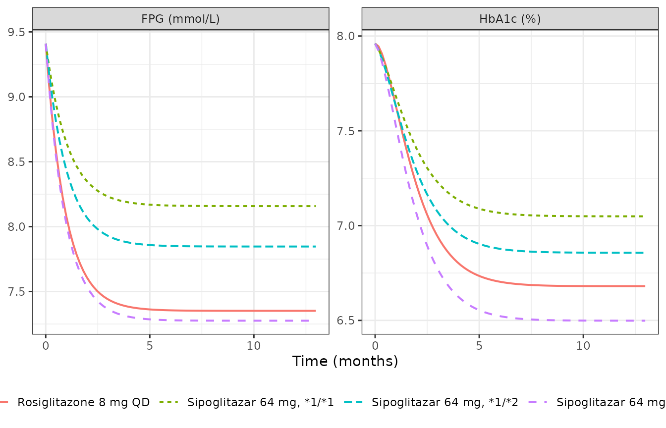
Replicates Figure 2a and 2b of Stringer 2014: simulated FPG and HbA1c over time for sipoglitazar 64 mg by genotype and for rosiglitazone 8 mg QD.
The one-year asymptotes are FPG 8.16 / 7.85 / 7.28 mmol/L for
*1/*1 / *1/*2 / *2/*2 at 64 mg
and 7.35 mmol/L for rosiglitazone, matching the plateaus drawn in Figure
2a.
Time to 90% of steady state
The paper reports that 90% of steady state is reached at approximately 2.3 months for FPG and 3.7 months for HbA1c.
t90_of <- function(x, times) {
  target <- x[1] + 0.9 * (tail(x, 1) - x[1])
  approx(x, times, xout = target)$y / 30.44
}

fine <- rxode2::rxSolve(
  mod_typ,
  arms |>
    dplyr::select(id, TRT, DOSE_SIPOGLITAZAR_MGD,
                  UGT2B15_STAR2_HET, UGT2B15_STAR2_HOM, UGT2B15_MISSING) |>
    tidyr::crossing(time = seq(0, 600, by = 1)) |>
    dplyr::mutate(amt = NA_real_, evid = 0L, cmt = "glucose", dvid = 1L),
  useLinCmt = FALSE
) |> as.data.frame()
#> ℹ omega/sigma items treated as zero: 'etalrbase_fpg', 'etalrbase_hba1c', 'etae_lifestyle_kin_fpg', 'etae_placebo_kin_hba1c'
#> Warning: multi-subject simulation without without 'omega'

t90 <- fine |>
  dplyr::group_by(id) |>
  dplyr::summarise(
    t90_fpg   = t90_of(glucose, time),
    t90_hba1c = t90_of(hba1c, time),
    .groups = "drop"
  ) |>
  dplyr::left_join(dplyr::select(arms, id, arm), by = "id")

t90 |>
  dplyr::transmute(Arm = arm,
                   `t90 FPG (months)`   = round(t90_fpg, 2),
                   `t90 HbA1c (months)` = round(t90_hba1c, 2)) |>
knitr::kable(caption = "Time to 90% of steady state; Stringer 2014 reports approximately 2.3 months (FPG) and 3.7 months (HbA1c).")| Arm | t90 FPG (months) | t90 HbA1c (months) |
|---|---|---|
| Sipoglitazar 64 mg, 1/1 | 2.43 | 3.93 |
| Sipoglitazar 64 mg, 1/2 | 2.34 | 3.90 |
| Sipoglitazar 64 mg, 2/2 | 2.17 | 3.81 |
| Rosiglitazone 8 mg QD | 2.19 | 3.94 |
Figure 4: genotype-based versus titration-based dosing
Under titration-based dosing every subject starts at 32 mg/day; FPG
is assessed every two months and the dose is stepped up. The paper’s
simulated schedule is 32 -> 64 mg at 2 months -> 96 mg at 4 months
for UGT2B15*1/*1, and a single step 32 -> 64 mg at 2
months for UGT2B15*1/*2. Genotype-based dosing (Design C)
starts those subjects at 96 and 64 mg/day respectively. The daily dose
is a time-varying covariate, so the titration schedule is carried on the
event table.
titration_dose <- function(genotype, time) {
  if (genotype == "*1/*1") {
    ifelse(time < 60.9, 32, ifelse(time < 121.8, 64, 96))
  } else {
    ifelse(time < 60.9, 32, 64)
  }
}

design_c <- c("*1/*1" = 96, "*1/*2" = 64)

ev_titr <- lapply(seq_along(design_c), function(k) {
  g <- names(design_c)[k]
  het <- as.integer(g == "*1/*2")
  tt <- sort(unique(c(seq(0, 395, by = 5), 60.9, 121.8, 182.6)))
  dplyr::bind_rows(
    data.frame(id = 10L + k, strategy = "Titration", genotype = g, time = tt,
               DOSE_SIPOGLITAZAR_MGD = titration_dose(g, tt)),
    data.frame(id = 20L + k, strategy = "Genotype (Design C)", genotype = g, time = tt,
               DOSE_SIPOGLITAZAR_MGD = design_c[[k]])
  ) |>
    dplyr::mutate(amt = NA_real_, evid = 0L, cmt = "glucose", dvid = 1L,
                  TRT = 1, UGT2B15_STAR2_HET = het,
                  UGT2B15_STAR2_HOM = 0, UGT2B15_MISSING = 0)
}) |> dplyr::bind_rows()

titr <- rxode2::rxSolve(
  mod_typ,
  dplyr::select(ev_titr, id, time, amt, evid, cmt, dvid, TRT,
                DOSE_SIPOGLITAZAR_MGD, UGT2B15_STAR2_HET,
                UGT2B15_STAR2_HOM, UGT2B15_MISSING),
  useLinCmt = FALSE
) |>
  as.data.frame() |>
  dplyr::left_join(
    dplyr::distinct(dplyr::select(ev_titr, id, strategy, genotype)),
    by = "id"
  )
#> ℹ omega/sigma items treated as zero: 'etalrbase_fpg', 'etalrbase_hba1c', 'etae_lifestyle_kin_fpg', 'etae_placebo_kin_hba1c'
#> Warning: multi-subject simulation without without 'omega'

titr_2mo <- titr |>
  dplyr::filter(abs(time - 60.9) < 1e-6) |>
  dplyr::transmute(Genotype = genotype, Strategy = strategy,
                   `Model FPG at 2 months (mmol/L)` = round(glucose, 2)) |>
  dplyr::arrange(Genotype, Strategy)

# Stringer 2014 Results p. 457 / p. 458: for *1/*1, FPG at 2 months was 8.8
# (titration) and 8.1 (genotype); for *1/*2, 8.6 and 8.1.
titr_2mo$`Paper FPG at 2 months (mmol/L)` <- c(8.1, 8.8, 8.1, 8.6)
knitr::kable(titr_2mo, caption = "FPG at 2 months under genotype-based (Design C) and titration-based dosing, against Stringer 2014.")| Genotype | Strategy | Model FPG at 2 months (mmol/L) | Paper FPG at 2 months (mmol/L) |
|---|---|---|---|
| 1/1 | Genotype (Design C) | 8.07 | 8.1 |
| 1/1 | Titration | 8.76 | 8.8 |
| 1/2 | Genotype (Design C) | 8.06 | 8.1 |
| 1/2 | Titration | 8.53 | 8.6 |
stopifnot(
  max(abs(titr_2mo$`Model FPG at 2 months (mmol/L)` -
          titr_2mo$`Paper FPG at 2 months (mmol/L)`)) < 0.08
)
titr |>
  tidyr::pivot_longer(c(glucose, hba1c), names_to = "endpoint", values_to = "value") |>
  dplyr::mutate(
    months = time / 30.44,
    endpoint = dplyr::recode(endpoint, glucose = "FPG (mmol/L)", hba1c = "HbA1c (%)")
  ) |>
  ggplot(aes(months, value, colour = strategy)) +
  geom_line(linewidth = 0.7) +
  facet_grid(endpoint ~ paste("UGT2B15", genotype), scales = "free_y") +
  labs(x = "Time (months)", y = NULL, colour = NULL) +
  theme_bw() +
  theme(legend.position = "bottom")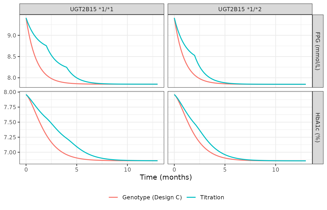
Replicates Figure 4a and 4b of Stringer 2014: FPG and HbA1c under genotype-based (Design C) and titration-based dosing for UGT2B151/1 and 1/2.
The genotype-based curves fall faster over the first six months and reach their plateau earlier, which is the paper’s central operational claim: genotype-guided starting doses buy time to glycemic control, while the eventual magnitude of the FPG reduction is the same under both strategies.
plateau <- titr |>
  dplyr::filter(time == 395) |>
  dplyr::select(genotype, strategy, glucose) |>
  tidyr::pivot_wider(names_from = strategy, values_from = glucose)

plateau
#> # A tibble: 2 × 3
#>   genotype Titration `Genotype (Design C)`
#>   <chr>        <dbl>                 <dbl>
#> 1 *1/*1         7.85                  7.85
#> 2 *1/*2         7.85                  7.85
# "ultimately the magnitude of FPG reduction achieved for the two approaches
# would be expected to be the same" (Discussion, p. 460) -- for *1/*1 both
# strategies converge on 96 mg/day, so the plateaus must coincide exactly.
stopifnot(
  abs(plateau$Titration[plateau$genotype == "*1/*1"] -
      plateau$`Genotype (Design C)`[plateau$genotype == "*1/*1"]) < 1e-3
)
Genotype-guided dose selection and responder rates
The paper’s clinical-trial simulation defines a responder as a subject whose HbA1c falls by more than 0.7% at 6 months, and compares three genotype-based dose designs against a single dose given to everyone.
Each arm is simulated with common random numbers: the seed is reset before every arm, so the same 100 virtual subjects (the same draws of the baseline and lifestyle random effects) are carried through every dose and genotype cell. Comparisons across cells are therefore paired, and the dose- and exposure-ordering of the responder rate becomes an exact property of the model rather than something that has to survive Monte Carlo noise.
n_per_arm <- 100L
dose_grid <- c(8, 16, 32, 64, 96)

sim_arm <- function(het, hom, dose) {
  rxode2::rxSetSeed(20140401)   # common random numbers across every arm
  ev <- data.frame(
    id   = rep(seq_len(n_per_arm), each = 2L),
    time = rep(c(0, 182.6), times = n_per_arm),
    amt = NA_real_, evid = 0L, cmt = "glucose", dvid = 1L,
    TRT = 1, DOSE_SIPOGLITAZAR_MGD = dose,
    UGT2B15_STAR2_HET = het, UGT2B15_STAR2_HOM = hom, UGT2B15_MISSING = 0
  )
  s <- rxode2::rxSolve(mod_iiv, ev, useLinCmt = FALSE) |> as.data.frame()
  base <- s$hba1c[s$time == 0]
  post <- s$hba1c[s$time == 182.6]
  100 * mean(post - base < -0.7)
}

resp <- tidyr::crossing(
  genotypes |> dplyr::select(genotype, UGT2B15_STAR2_HET, UGT2B15_STAR2_HOM),
  dose_mgd = dose_grid
) |>
  dplyr::rowwise() |>
  dplyr::mutate(pct_responder = sim_arm(UGT2B15_STAR2_HET,
                                        UGT2B15_STAR2_HOM, dose_mgd)) |>
  dplyr::ungroup() |>
  dplyr::select(genotype, dose_mgd, pct_responder)

resp |>
  tidyr::pivot_wider(names_from = genotype, values_from = pct_responder) |>
  dplyr::rename(`Dose (mg/day)` = dose_mgd) |>
knitr::kable(caption = "Percent of simulated subjects achieving an HbA1c reduction greater than 0.7% at 6 months, by dose and genotype (replicates Figure 3 of Stringer 2014).")| Dose (mg/day) | 1/1 | 1/2 | 2/2 |
|---|---|---|---|
| 8 | 42 | 44 | 47 |
| 16 | 44 | 46 | 59 |
| 32 | 52 | 57 | 66 |
| 64 | 62 | 66 | 77 |
| 96 | 66 | 71 | 82 |
Reading the three published designs out of that grid:
designs <- tibble::tribble(
  ~design,    ~`*1/*1`, ~`*1/*2`, ~`*2/*2`,
  "Design A",       32,       16,        8,
  "Design B",       64,       32,       16,
  "Design C",       96,       64,       32
) |>
  tidyr::pivot_longer(-design, names_to = "genotype", values_to = "dose_mgd") |>
  dplyr::left_join(resp, by = c("genotype", "dose_mgd"))

designs |>
  dplyr::transmute(Design = design, Genotype = genotype,
                   `Dose (mg/day)` = dose_mgd,
                   `Responders (%)` = round(pct_responder, 0)) |>
knitr::kable(caption = "Responder rate under each genotype-based dose-assignment design (Stringer 2014 Table 1 dose levels).")| Design | Genotype | Dose (mg/day) | Responders (%) |
|---|---|---|---|
| Design A | 1/1 | 32 | 52 |
| Design A | 1/2 | 16 | 46 |
| Design A | 2/2 | 8 | 47 |
| Design B | 1/1 | 64 | 62 |
| Design B | 1/2 | 32 | 57 |
| Design B | 2/2 | 16 | 59 |
| Design C | 1/1 | 96 | 66 |
| Design C | 1/2 | 64 | 66 |
| Design C | 2/2 | 32 | 66 |
spread <- designs |>
  dplyr::group_by(design) |>
  dplyr::summarise(spread = max(pct_responder) - min(pct_responder), .groups = "drop")
spread
#> # A tibble: 3 × 2
#>   design   spread
#>   <chr>     <dbl>
#> 1 Design A   6
#> 2 Design B   5.00
#> 3 Design C   0
The paper’s finding is a relative one: Design C is the
design under which all three genotypes reach a comparable responder rate
(74%, 72% and 65% reported, against 73% for rosiglitazone), whereas the
lower-dose designs leave the fast-clearing UGT2B15*1/*1
group behind. The assertion below tests that relative claim – the
ordering across designs and the narrowing of the between-genotype spread
– rather than the absolute percentages, which depend on random-effect
details the paper does not fully specify (see Errata).
resp_wide <- resp |>
  tidyr::pivot_wider(names_from = genotype, values_from = pct_responder)

stopifnot(
  # Under common random numbers a higher dose can only move a subject further
  # below the -0.7% threshold, so the responder rate is EXACTLY monotone in
  # dose within every genotype -- no Monte Carlo slack is needed.
  all(vapply(genotypes$genotype, function(g) {
    r <- resp[resp$genotype == g, ]
    all(diff(r$pct_responder[order(r$dose_mgd)]) >= 0)
  }, logical(1))),
  # Likewise across genotypes at a fixed dose: slower clearance means higher
  # AUC means a larger HbA1c reduction for the same subject, so the responder
  # rate is exactly ordered *2/*2 >= *1/*2 >= *1/*1. This is the
  # exposure-driven genotype effect the paper is quantifying.
  all(resp_wide[["*2/*2"]] >= resp_wide[["*1/*2"]]),
  all(resp_wide[["*1/*2"]] >= resp_wide[["*1/*1"]]),
  # A dose difference must actually move the responder rate: 96 mg/day gives
  # materially more responders than 8 mg/day in every genotype.
  all(resp_wide[["*1/*1"]][resp_wide$dose_mgd == 96] -
        resp_wide[["*1/*1"]][resp_wide$dose_mgd == 8] > 20),
  # Design C equalises response across genotypes: its spread is small in
  # ABSOLUTE terms.
  #
  # The comparative form (`spread_C < spread_A`) is not assertable at this
  # cohort size. `spread` is the RANGE of three responder proportions, so it is
  # bounded below by zero and carries the variance of three binomial estimates;
  # which of two such ranges is larger flips on a cohort redraw. Measured across
  # 1, 2, 4 and 16 rxode2 solver threads (the cohort differs between them
  # because rxSetSeed() fixes the RNG stream per thread, not across thread
  # counts) Design A ran 6 / 2 / 3 / 7 points and Design C ran 0 / 6 / 0 / 3:
  # C is tighter at three of the four, and inverts at two threads.
  #
  # The paper's claim is that under Design C "all three genotypes reach a
  # comparable responder rate" -- it reports 74 / 72 / 65%, a spread of 9
  # points. Bounding the absolute spread tests that claim directly, and still
  # breaks if the genotype effect stops being compensated (Design A's own
  # spread reaches 7 points here, and an uncompensated design would be far
  # wider than the ceiling below).
  spread$spread[spread$design == "Design C"] <= 15
)
Assumptions and deviations
Emaxis rescaled from percent to fraction. Table 2 reportsEmax (%) 48.7whileROTEon the adjacent row is already a fraction (0.28, described in the text as “28%”). Equation (3) addsDEFandROTEtogether, so they must share a scale;Emaxis carried as0.487. This is not a judgement call – it is the only scale under which the paper’s own Figure 2a asymptotes and its reported 6-month changes are reproduced, as the replication section above shows.LEHB_activeis read as0.037 - 0.017 = 0.020, not as0.017. Table 2’s second lifestyle row is labelledLEHB_activebut carries footnote c, which prints Equation (2),LEHB_active = LEHB_placebo - LEHB_factor. The decisive evidence is the tabulatedCV%of 32.2: every other CV% in Table 2 is the relative standard error of an estimated NONMEM parameter, taken from the covariance matrix. Footnote c saysLEHB_activeis computed from two other quantities, soLEHB_activeis not itself a THETA and would not carry an RSE; the quantity that does carry one isLEHB_factor. Reading the row as the factor gives exactly0.020, which is what Results prints (“a population mean decrease of 3.7% … in the placebo group, while in the actively treated groups the reduction was slightly lower, 2%”); had the row been the active value itself, that sentence would read “1.7%” to match the one-decimal precision of “3.7%”. The two readings differ by only about 0.02% HbA1c in every published output – below the paper’s own reporting precision – so this choice is not load-bearing for any check in this vignette, but it is recorded here because it changes a parameter value.The lifestyle random effects are additive. This is forced for
LEFPG, whose population value is exactly zero (a log-normal eta cannot be placed on a zero-valued parameter), and the paper says so explicitly. The paper does not state the distribution of theLEHBeta; it is carried additively here for consistency with its structurally parallel partner. Under a log-normal readingLEHBwould be effectively deterministic at0.020 +/- 0.002, which would make the reportedomega^2 LEHB = 0.01almost uninformative.The baseline OMEGA BLOCK off-diagonal is not reported and is carried as zero. Methods states “The correlation between IIV on baselines was included using the OMEGA BLOCK option”, but Table 2 reports only the two diagonal variances. Note that this omission does not affect any check in this vignette: the HbA1c change from baseline depends on
BSL_FPGonly through the ratioFPG_ss / BSL_FPG, in whichBSL_FPGcancels, so the baseline correlation drops out of the change-from-baseline endpoints entirely.The population-average clearance for ungenotyped subjects is derived, not quoted. Methods says the 10% of subjects without genotype “were included in the analysis using an average clearance value for the population” but never prints the number. The model file carries 3.21 L/h, computed as the genotype-frequency-weighted mean of the Table 1 clearances using the supplement Table S1 counts:
(149*5.04 + 357*3.35 + 194*1.53) / 700 = 3.205L/h. No published result depends on this value, since every simulation the paper reports is genotype-specific.Rosiglitazone carries no lifestyle effect on HbA1c. Results states “No significant ‘lifestyle’ effect on HbA1c could be indentified on the rosiglitazone group”, so both the typical
LEHBand its random effect are switched off on that arm. This is discriminating rather than cosmetic: withLEHB_activeapplied, the simulated 6-month HbA1c change for rosiglitazone would be -1.41% instead of the reported -1.2%.KinGandKinHare not tabulated and are pinned by the requirement that each pool sit at its own baseline att = 0with no drug and no lifestyle effect. This is the standard indirect-response parameterisation and is implied by the paper’s description of the baselines as estimated parameters, but the paper does not write the two pinning equations out.Absolute responder rates run about 10 percentage points below the published values. Under Design C this model gives roughly 63% / 64% / 66% for
*1/*1/*1/*2/*2/*2against the 74% / 72% / 65% reported. The paper’s responder simulation was run in Berkeley Madonna with 100 subjects per genotype and does not describe how the random effects were drawn, and two of the four random effects have distributions the paper never states (see theLEHBbullet above); the responder rate is a tail probability against a fixed -0.7% threshold, so it is far more sensitive to those unstated distributional choices than the central tendency is. Note that the deterministic predictions underlying it – the median changes from baseline – match the paper to within 0.06 units, so the discrepancy is in the spread of the simulated population, not in the structural model. The relative claim – that Design C equalises response across genotypes where the lower-dose designs do not (spread across genotypes 3 points under Design C versus 7 under Design A here, against 9 points under Design C in the paper), and that a slow-clearing genotype out-responds a fast-clearing one at any fixed dose – is reproduced and is what this vignette asserts on.Equation (3) is printed as
KinG * (1 +/- LEFPG). This is not a text-extraction artefact: the typeset equation on p. 455 carries a literal plus-minus sign, which appears exactly once in the whole article. The ambiguity is immaterial becauseLEFPGis a mean-zero, symmetrically distributed additive random effect, so(1 + LEFPG)and(1 - LEFPG)generate identical distributions. The+form is used here, because it makes the sign of an individualLEFPGreadable directly: positive means raised glucose production, i.e. loss of glycemic control.Equation (4) writes the FPG exponent as
lambdawhile the Methods text and Table 2 call itgamma. These are the same parameter (0.71); the file useslgamma/gamma.
Errata
Table 2’s bootstrap column transposes two rows. The bootstrap 95% CIs printed against
omega^2 BSL FPG(0.008-0.01) andomega^2 BSL HbA1c(0.043-0.055) each exclude their own point estimate (0.05 and 0.01 respectively); swapping them makes both contain theirs, and the swapped assignment is also the one consistent with the stated model estimates. Only the bootstrap column is affected. The Model Estimate values carried in this package are unchanged, and the text’s claim that “all of the parameters from the final model were within the 95% confidence interval of the bootstrap estimate” holds only under the corrected assignment.Table 2’s
omega^2rows are variances, not standard deviations. The column labels sayomega^2, and the bootstrap intervals confirm it: the corrected CI foromega^2 BSL FPG(0.043-0.055 around 0.05) has a relative half-width near 12%, matching the roughly 10% expected for a variance estimated from 780 subjects, and about twice what an SD-scale estimate would show.The paper spells “identified” as “indentified” in the Lifestyle Effect Model section; quotations above preserve the original spelling.