Efineptakin alfa (Jeon 2025)

library(nlmixr2lib)
library(rxode2)
#> rxode2 5.1.8 using 2 threads (see ?getRxThreads)
#>   no cache: create with `rxCreateCache()`
library(dplyr)
#> 
#> Attaching package: 'dplyr'
#> The following objects are masked from 'package:stats':
#> 
#>     filter, lag
#> The following objects are masked from 'package:base':
#> 
#>     intersect, setdiff, setequal, union
library(tidyr)
library(ggplot2)
library(PKNCA)
#> 
#> Attaching package: 'PKNCA'
#> The following object is masked from 'package:stats':
#> 
#>     filter

Model and source

• Citation: Jeon HS, Lee SW, Jung W, Jung H, Choi D, Byun M-S, Yun H-y, Lee S, Kim A, Chae J-w, Lee H. Dose Optimization of rhIL-7-hyFc for Patients With Lymphopenia Using a Neonatal Fc Receptor-Mediated Recycling-Based and Target-Mediated Drug Disposition Pharmacokinetic Model. Clin Transl Sci. 2025;18(5):e70252. doi:10.1111/cts.70252. PMCID: PMC12094080.
• Description: Semi-mechanistic population PK model for efineptakin alfa (rhIL-7-hyFc, GX-I7 / NT-I7; a homodimer of two IL-7 moieties fused to a hybrid IgD/IgG4 Fc, 104 kDa) after a single SC or IM microdose in healthy adults. Three states: the dose enters an injection-site / interstitial absorption space (apparent volume V_I, route-specific) that exchanges bidirectionally with central (Q) and is taken up (k_uptake) into a lumped FcRn-recycling endosomal space (apparent volume V_D). In the endosome the drug binds FcRn at quasi-steady state and the complex leaves at k_recycle, a fraction FR = 0.715 returning to central and the rest to the injection site. In central the drug binds IL-7R (CD127) at quasi-steady state (QSS-TMDD) with internalisation k_int and is cleared linearly (CL). Amounts are pmol of IL-7 (two per drug molecule); the observation is the free central IL-7 concentration (pmol/L).
• Article: https://doi.org/10.1111/cts.70252 (open access; Supporting Information Text S1 is the final NONMEM control stream and Table S1 the provenance of the fixed parameters)
• Primary trial report (demographics and NCA used below): Lee SW et al. Clin Transl Sci 2020;13:1161-1169, https://doi.org/10.1111/cts.12800

Efineptakin alfa (rhIL-7-hyFc; development codes GX-I7 and NT-I7) is a homodimer of two recombinant human IL-7 molecules fused to a hybrid IgD/IgG4 Fc (“hyFc”), 104 kDa. The Fc lets it bind the neonatal Fc receptor (FcRn) and escape lysosomal catabolism. Jeon et al. (2025) fitted a semi-mechanistic model to the microdose phase 1 trial in healthy adults and used it to propose IM dosing regimens for lymphopenia.

The model has three states:

• abs_site – the injection-site / interstitial space that receives the SC or IM dose. It exchanges with central in both directions (Q / V_I out, Q / V_C on free drug back) and feeds the endosome at k_uptake. The apparent volume V_I is route-specific (ROUTE_SC).
• central – serum. Drug binds IL-7R (CD127) at quasi-steady state (QSS-TMDD, R_tot = 1360 pmol/L); the complex is internalised at k_int and free drug is cleared at CL.
• endosome – a lumped FcRn-recycling endosomal space (apparent volume V_D). Drug binds FcRn (92 uM) at quasi-steady state; the complex leaves at k_recycle, 71.5 % to central and the rest back to the injection site.

All amounts are pmol of IL-7: the drug is dosed in pmol of rhIL-7-hyFc and f(abs_site) = 2 counts its two IL-7 moieties. The observation Cc is the free IL-7 concentration in serum (pmol/L), which the authors assumed the baseline-adjusted ELISA measured.

Population

The model was fitted to 410 baseline-adjusted serum IL-7 concentrations from 24 healthy adults in the randomized, double-blind, placebo-controlled phase 1 trial NCT02860715 (Seoul National University Hospital). Thirty subjects were randomized 8:2 to drug or placebo in three single-dose cohorts: 20 ug/kg SC, 60 ug/kg SC and 60 ug/kg IM (8 active subjects per cohort). Jeon 2025 does not tabulate demographics; the trial report (Lee 2020) gives mean +/- SD age 27.1 +/- 6.0 years, height 1.70 +/- 0.08 m, weight 65.3 +/- 11.1 kg and BMI 22.4 +/- 2.4 kg/m^2, with men and women 19-45 years eligible. Stepwise covariate modelling of age, sex, weight, height and BMI retained no covariate, which the authors attribute to weight-based dosing.

str(readModelDb("Jeon_2025_efineptakin_alfa")()$population)
#> List of 13
#>  $ species       : chr "human"
#>  $ n_subjects    : num 24
#>  $ n_studies     : num 1
#>  $ n_observations: num 410
#>  $ study_id      : chr "NCT02860715 (phase 1, randomized, double-blind, placebo-controlled; Seoul National University Hospital)"
#>  $ age_range     : chr "19-45 years (eligibility); mean 27.1 +/- 6.0 years (Lee 2020)"
#>  $ weight_range  : chr "mean 65.3 +/- 11.1 kg (Lee 2020)"
#>  $ sex_female_pct: logi NA
#>  $ race_ethnicity: chr "Korean (single-centre study in the Republic of Korea; not tabulated)"
#>  $ disease_state : chr "Healthy adult volunteers"
#>  $ dose_range    : chr "Single dose of rhIL-7-hyFc 20 ug/kg SC, 60 ug/kg SC or 60 ug/kg IM (8 active subjects per cohort; 30 randomized"| __truncated__
#>  $ regions       : chr "Republic of Korea"
#>  $ notes         : chr "Demographics are not reported in Jeon 2025, which refers to the primary trial report (Lee SW et al., Clin Trans"| __truncated__

Source trace

Every value is the final estimate in the Text S1 control stream, and every estimated value equals the “Observed value - Median” column of Table 1.

Equation / parameter	Value	Source location
lcl (CL)	8.91 L/h	Text S1 $THETA 1; Table 1
lvc (V_C)	39 L	Text S1 $THETA 2; Table 1
lq (Q)	5.46 L/h	Text S1 $THETA 3; Table 1
lkup (k_uptake)	0.00952 1/h, fixed	Text S1 $THETA 4 (FIX); Table S1 (Waldmann 1990)
lvendosome (V_D)	0.138 L	Text S1 $THETA 5; Table 1
lkrec (k_recycle)	0.00107 1/h	Text S1 $THETA 6; Table 1
lkint (k_int)	0.375 1/h	Text S1 $THETA 7 (estimated, not FIX); Table 1
lc_il7r_t (R_tot)	1360 pmol/L, fixed	Text S1 $THETA 8 (FIX); Table S1 (Monti 2013 Figure 3E)
lvabs_im (V_I, IM)	442 L	Text S1 $THETA 11; Table 1
lvabs_sc (V_I, SC)	1680 L	Text S1 $THETA 12; Table 1
c_fcrn_t (FcRn)	91,950,000 pmol/L, fixed	Text S1 $PK; Table S1 (Barber 2023)
fr_recycle (FR)	0.715, fixed	Text S1 $PK; Table S1 (Zhao 2013, Garg 2007)
koff_fcrn, kon_fcrn	12.132 1/h, 4.068e-4 L/pmol/h	Text S1 $PK (KOFF1, KON1); Methods 2.1 (biolayer interferometry)
koff_il7r, kon_il7r	59.76 1/h, 2.0196e-3 L/pmol/h	Text S1 $PK (KOFF2, KON2)
etalcl	0.347 (64.4 % CV)	Text S1 $OMEGA 1; Table 1
etalq	0.659 (96.6 % CV)	Text S1 $OMEGA 2; Table 1
propSd	0.335	Text S1 $THETA 9; Table 1
addSd	1.05 pmol/L	Text S1 $THETA 10; Table 1
kss_fcrn, kss_il7r	(k_recycle + k_off1)/k_on1, (k_int + k_off2)/k_on2	Eqs. (1), (2); Text S1 $PK
QSS free concentration	quadratic root	Text S1 $DES, $ERROR
d/dt(abs_site), d/dt(central), d/dt(endosome)	–	Text S1 $DES DADT(1)-DADT(3); Figure 1
f(abs_site) = 2	–	Text S1 $PK F1 = 2, dataset note “AMT: GX-I7 pmol x 2 = IL7 pmol”
ROUTE_SC switch on V_I	–	Text S1 $PK VI = VISC; IF(COHORT.EQ.3) VI = VIIM
Cc ~ prop() + add() on free conc.	–	Text S1 $ERROR, $SIGMA 1 FIX

mod <- readModelDb("Jeon_2025_efineptakin_alfa")

# ug/kg of rhIL-7-hyFc -> pmol of drug (MW 104 kDa; Methods 2.1)
dose_pmol <- function(ug_per_kg, wt) ug_per_kg * wt * 1e-6 / 104000 * 1e12

# ug/L of IL-7 -> pmol/L (20.5 kDa per IL-7 moiety; Methods 2.1)
ugL_to_pM <- function(x) x * 1e-6 / 20500 * 1e12

# Weight drawn from the trial mean and SD (Lee 2020), as Jeon 2025 describes
# for its own simulations; redraw the rare non-physiological low tail.
draw_wt <- function(n) {
  wt <- rnorm(n, 65.3, 11.1)
  while (any(low <- wt < 40)) wt[low] <- rnorm(sum(low), 65.3, 11.1)
  wt
}

# The study's three cohorts
cohorts <- tibble::tribble(
  ~cohort,          ~dose_ugkg, ~ROUTE_SC,
  "20 ug/kg s.c.",  20,         1,
  "60 ug/kg i.m.",  60,         0,
  "60 ug/kg s.c.",  60,         1
)

Structural checks (typical subject)

Two identities must hold exactly for any correct implementation, so they are checked on a typical-value solve at tight tolerances. The cumulative amount eliminated (linear clearance plus IL-7R-complex internalisation) is tracked with an extra state appended to the model for this check only.

ui_mb <- rxode2::rxode2(mod) |>
  rxode2::model(
    {
      d/dt(auc_central) <- Cc
      d/dt(eliminated) <- kel * c_free * vc + kint * c_cpx * vc
    },
    append = TRUE
  )
#> ℹ parameter labels from comments will be replaced by 'label()'
# An explicit ODE model: rxode2 must not have replaced it by linCmt()
stopifnot(is.null(rxode2::rxode2(mod)$linCmt))
#> ℹ parameter labels from comments will be replaced by 'label()'

ev_mb <- rxode2::et(amt = dose_pmol(60, 65.3), cmt = "abs_site") |>
  rxode2::et(seq(0, 30000, by = 10)) |>
  as.data.frame() |>
  mutate(ROUTE_SC = 0)
typ_mb <- rxode2::rxSolve(
  rxode2::zeroRe(ui_mb), ev_mb,
  rtol = 1e-10, atol = 1e-12, maxsteps = 1e6, returnType = "data.frame"
)
#> ℹ omega/sigma items treated as zero: 'etalcl', 'etalq'
f_in <- 2 * dose_pmol(60, 65.3)

checks <- typ_mb |>
  filter(time > 0) |>
  summarise(
    mass_balance_relerr = max(abs(
      (abs_site + central + endosome + eliminated) / f_in - 1
    )),
    qss_central_relerr = max(abs((c_free + c_cpx) / c_tot - 1)),
    qss_endosome_relerr = max(abs((a_free + a_cpx) / a_tot - 1)),
    max_free_over_total = max(c_free / c_tot),
    remaining_at_30000h = last(abs_site + central + endosome) / f_in
  )
tibble(check = names(checks), value = formatC(unlist(checks), format = "g", digits = 3)) |>
  knitr::kable()

check	value
mass_balance_relerr	3.11e-15
qss_central_relerr	4.44e-16
qss_endosome_relerr	4.44e-16
max_free_over_total	0.956
remaining_at_30000h	1.49e-10

stopifnot(
  # Every pmol dosed (x2 IL-7 moieties) is in a state or has been eliminated.
  # Measured ~3e-15; a missing or mis-signed flux term moves this by > 1e-3.
  checks$mass_balance_relerr < 1e-8,
  # The rationalised QSS root reproduces the total exactly in both spaces.
  checks$qss_central_relerr < 1e-8,
  checks$qss_endosome_relerr < 1e-8,
  checks$max_free_over_total <= 1
)

At microdose and therapeutic concentrations IL-7R binding is far from saturation (free concentration is almost all of the total; R_tot is small against K_SS2), so total exposure follows the linear identity AUC(free) x (CL + k_int x V_C x R_tot / K_SS2) = 2 x Dose:

p_typ <- typ_mb[1, ]
cl_eff <- p_typ$cl + p_typ$kint * p_typ$vc * p_typ$c_il7r_t / p_typ$kss_il7r
auc_ratio <- last(typ_mb$auc_central) * cl_eff / f_in
auc_ratio
#> [1] 1.000036
# Measured 0.9999+: the only departure is the tiny non-linearity of the
# IL-7R term, so 1 % separates it from any error in CL, V_C or the dose units.
stopifnot(abs(auc_ratio - 1) < 0.01)

The slow phase is the endosomal recycling (k_recycle = 0.00107 1/h, a ~650 h half-life), so only about two thirds of this total exposure accrues within the 672 h sampling window of the trial.

Virtual cohort and simulation

Each of the three study cohorts is simulated with 200 subjects (the trial had 8 per cohort) at the trial’s sampling times (Lee 2020: 0, 1, 2, 4, 6, 8, 11, 14, 24, 36, 48, 60, 72, 96, 168, 240, 336, 504 and 672 h) plus a dense grid for the figure.

# rxSetSeed() fixes the draw for a given solver thread count only; every
# assertion below is written to hold for any cohort the model can produce.
set.seed(20250252)
rxode2::rxSetSeed(20250252)

n_per_arm <- 200
pk_times <- c(0, 1, 2, 4, 6, 8, 11, 14, 24, 36, 48, 60, 72, 96, 168, 240, 336, 504, 672)
obs_times <- sort(unique(c(pk_times, seq(0, 672, by = 4))))

make_cohort <- function(k) {
  row <- cohorts[k, ]
  subj <- tibble(id = (k - 1L) * n_per_arm + seq_len(n_per_arm), WT = draw_wt(n_per_arm))
  dose <- subj |>
    mutate(time = 0, evid = 1L, cmt = "abs_site", amt = dose_pmol(row$dose_ugkg, WT))
  obs <- tidyr::expand_grid(subj, time = obs_times) |>
    mutate(evid = 0L, cmt = "central", amt = 0)
  bind_rows(dose, obs) |>
    mutate(cohort = row$cohort, ROUTE_SC = row$ROUTE_SC) |>
    arrange(id, time, desc(evid))
}
events <- bind_rows(lapply(seq_len(nrow(cohorts)), make_cohort))
stopifnot(!anyDuplicated(unique(events[, c("id", "time", "evid")])))

sim <- rxode2::rxSolve(mod, events = events, keep = c("cohort", "WT"),
                       returnType = "data.frame")
#> ℹ parameter labels from comments will be replaced by 'label()'
stopifnot(all(is.finite(sim$Cc)))

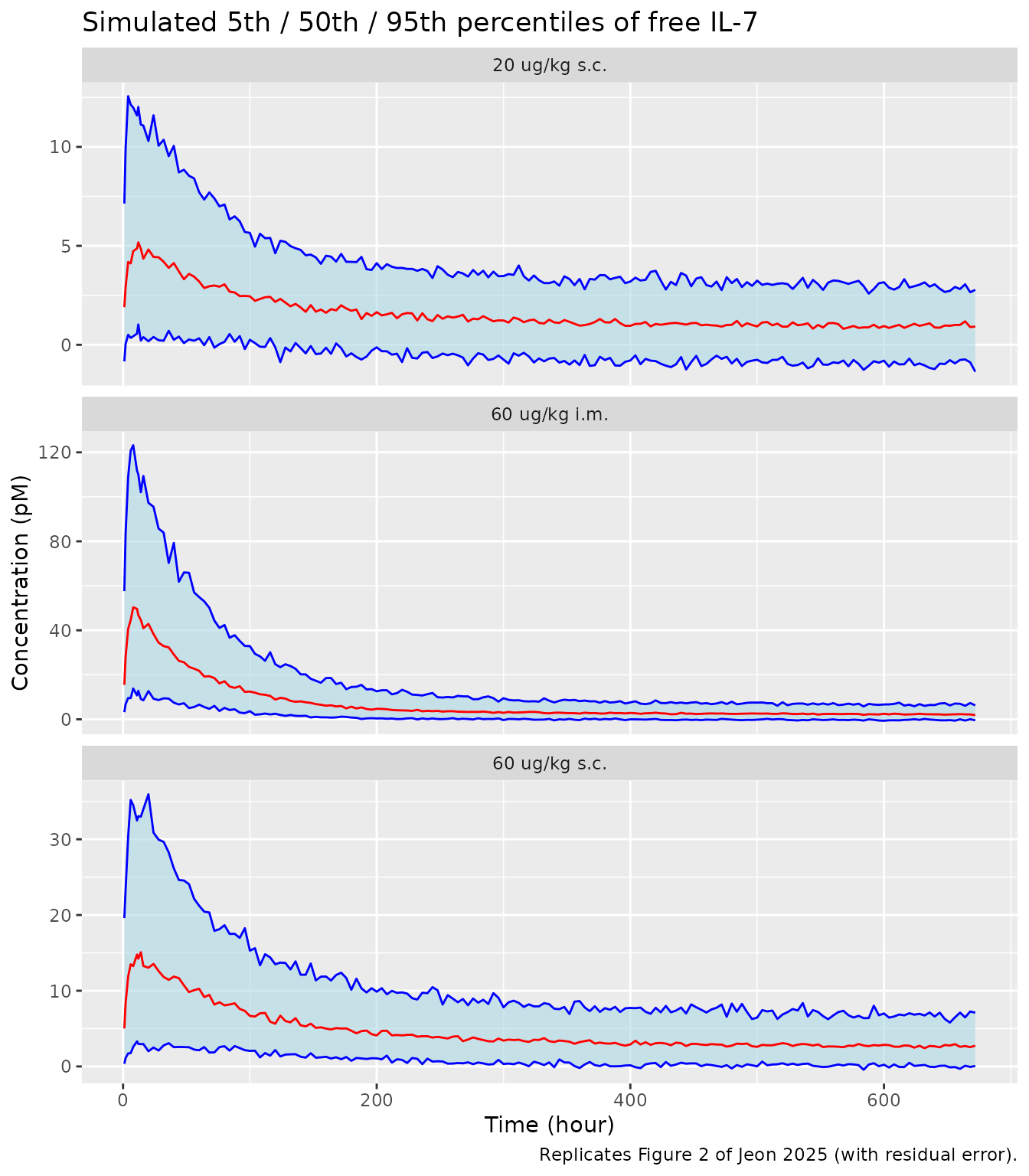
Replicate Figure 2 (VPC)

sim |>
  filter(time > 0) |>
  group_by(cohort, time) |>
  summarise(
    Q05 = quantile(sim, 0.05), Q50 = quantile(sim, 0.50), Q95 = quantile(sim, 0.95),
    .groups = "drop"
  ) |>
  ggplot(aes(time, Q50)) +
  geom_ribbon(aes(ymin = Q05, ymax = Q95), fill = "lightblue", alpha = 0.6) +
  geom_line(colour = "red") +
  geom_line(aes(y = Q05), colour = "blue") +
  geom_line(aes(y = Q95), colour = "blue") +
  facet_wrap(~cohort, ncol = 1, scales = "free_y") +
  labs(
    x = "Time (hour)", y = "Concentration (pM)",
    title = "Simulated 5th / 50th / 95th percentiles of free IL-7",
    caption = "Replicates Figure 2 of Jeon 2025 (with residual error)."
  )

sim |>
  filter(time > 0) |>
  group_by(cohort, time) |>
  summarise(Q50 = median(Cc), Q95 = quantile(Cc, 0.95), .groups = "drop") |>
  group_by(cohort) |>
  summarise(
    peak_median = max(Q50), time_of_peak_median = time[which.max(Q50)],
    peak_95th = max(Q95), .groups = "drop"
  ) |>
  dplyr::rename(
    "Cohort" = cohort, "Peak median Cc (pmol/L)" = peak_median,
    "Time of peak median (h)" = time_of_peak_median,
    "Peak 95th percentile (pmol/L)" = peak_95th
  ) |>
  knitr::kable(digits = 1)

Cohort	Peak median Cc (pmol/L)	Time of peak median (h)	Peak 95th percentile (pmol/L)
20 ug/kg s.c.	5.2	14	11.2
60 ug/kg i.m.	48.9	8	104.1
60 ug/kg s.c.	14.8	11	29.6

Figure 2 is a vector graphic, so the model-predicted confidence interval of the median (the red band) was digitised by the maintainers from the article PDF, calibrated on the panel gridlines, at the centre of each VPC time bin. The simulated median of the observations, pooled over the trial samples that fall in each bin, is compared with it below.

# Digitised from Jeon 2025 Figure 2 (red band = model-predicted CI of the
# median), pmol/L. Bin centres read from the band's vertices; the 60 ug/kg IM
# band at the two latest bins is hidden under the plotted lines.
band <- tibble::tribble(
  ~cohort,         ~bin_h, ~lower, ~upper,
  "20 ug/kg s.c.",  19,     2.33,   5.76,
  "20 ug/kg s.c.",  54,     1.88,   4.24,
  "20 ug/kg s.c.", 156,     1.08,   2.43,
  "20 ug/kg s.c.", 372,     0.81,   1.59,
  "20 ug/kg s.c.", 669,     0.52,   1.03,
  "60 ug/kg i.m.",  19,    25.94,  57.78,
  "60 ug/kg i.m.",  54,    13.79,  32.62,
  "60 ug/kg i.m.", 156,     4.72,  10.20,
  "60 ug/kg s.c.",  19,     7.86,  18.45,
  "60 ug/kg s.c.",  54,     6.13,  13.69,
  "60 ug/kg s.c.", 156,     3.72,   7.75,
  "60 ug/kg s.c.", 372,     2.21,   4.28,
  "60 ug/kg s.c.", 669,     1.87,   3.55
)
# Trial sampling times pooled into each bin
bin_times <- list(`19` = c(11, 14, 24), `54` = c(48, 60), `156` = 168,
                  `372` = c(336, 504), `669` = 672)
band_cmp <- band |>
  rowwise() |>
  mutate(sim_median = median(sim$sim[sim$cohort == cohort &
                                       sim$time %in% bin_times[[as.character(bin_h)]]])) |>
  ungroup() |>
  mutate(inside = sim_median >= lower & sim_median <= upper)
band_cmp |>
  dplyr::rename(
    "Cohort" = cohort, "Bin centre (h)" = bin_h,
    "Band lower (pmol/L)" = lower, "Band upper (pmol/L)" = upper,
    "Simulated median (pmol/L)" = sim_median, "Inside band" = inside
  ) |>
  knitr::kable(digits = 2)

Cohort	Bin centre (h)	Band lower (pmol/L)	Band upper (pmol/L)	Simulated median (pmol/L)	Inside band
20 ug/kg s.c.	19	2.33	5.76	4.75	TRUE
20 ug/kg s.c.	54	1.88	4.24	3.27	TRUE
20 ug/kg s.c.	156	1.08	2.43	1.74	TRUE
20 ug/kg s.c.	372	0.81	1.59	1.20	TRUE
20 ug/kg s.c.	669	0.52	1.03	0.92	TRUE
60 ug/kg i.m.	19	25.94	57.78	44.12	TRUE
60 ug/kg i.m.	54	13.79	32.62	23.84	TRUE
60 ug/kg i.m.	156	4.72	10.20	5.80	TRUE
60 ug/kg s.c.	19	7.86	18.45	14.45	TRUE
60 ug/kg s.c.	54	6.13	13.69	10.63	TRUE
60 ug/kg s.c.	156	3.72	7.75	5.06	TRUE
60 ug/kg s.c.	372	2.21	4.28	3.07	TRUE
60 ug/kg s.c.	669	1.87	3.55	2.74	TRUE

stopifnot(
  nrow(band_cmp) == 13, all(is.finite(band_cmp$sim_median)),
  # All 13 medians sat inside the band across repeated cohorts, the 20 ug/kg
  # late bin within 2 % of its upper edge; a 15 % margin absorbs the cohort
  # draw. The bands span about 2-fold, so a dose-unit error (2x), a wrong route
  # volume or a mis-placed recycling flux falls outside several of them.
  all(band_cmp$sim_median >= band_cmp$lower / 1.15),
  all(band_cmp$sim_median <= band_cmp$upper * 1.15)
)

The band itself shows the shape of the published model: after SC dosing the predicted median is highest in the first bin (about 19 h) and declines from there, while the observed median (red line in Figure 2) peaks in the 54 h bin. The early plateau and the slow tail at 2-4 pmol/L to 672 h are both reproduced, and they also explain the NCA comparison below.

NCA against the trial report

Lee 2020 (Table 1) reports NCA of the baseline-adjusted IL-7 concentrations by cohort, as mean +/- SD (Tmax as median) in ug/L of IL-7; they are converted here to pmol/L with the 20.5 kDa per IL-7 used by Jeon 2025. The trial’s NCA was run on measured concentrations, so the comparison uses simulated observations (the sim column, which carries the residual error) at the trial’s sampling times, and drops every sample below the assay’s lower limit of quantification (0.031 ng/mL = 1.51 pmol/L), as the trial could not have measured it. Noise matters here: after SC dosing the model predicts a broad plateau rather than a sharp peak, and on a plateau the observed Tmax is decided by assay noise.

lloq <- ugL_to_pM(0.031)

nca_conc <- sim |>
  filter(time %in% pk_times) |>
  transmute(id, time, cohort, Cc = if_else(time == 0, 0, sim)) |>
  filter(time == 0 | Cc >= lloq) |>
  arrange(id, time)
stopifnot(all(table(nca_conc$id[nca_conc$time == 0]) == 1))

nca_dose <- events |>
  filter(evid == 1) |>
  select(id, time, amt, cohort)

conc_obj <- PKNCA::PKNCAconc(nca_conc, Cc ~ time | cohort + id)
dose_obj <- PKNCA::PKNCAdose(nca_dose, amt ~ time | cohort + id)
intervals <- data.frame(
  start = 0, end = Inf,
  cmax = TRUE, tmax = TRUE, auclast = TRUE, aucinf.obs = TRUE, half.life = TRUE
)
nca_res <- PKNCA::pk.nca(PKNCA::PKNCAdata(conc_obj, dose_obj, intervals = intervals))
#> Warning: Too few points for half-life calculation (min.hl.points=3 with only 2
#> points)
#> Warning: Too few points for half-life calculation (min.hl.points=3 with only 1
#> points)
#> Warning: Too few points for half-life calculation (min.hl.points=3 with only 2
#> points)
#> Warning: Too few points for half-life calculation (min.hl.points=3 with only 0 points)
#> Too few points for half-life calculation (min.hl.points=3 with only 0 points)
#> Warning: Too few points for half-life calculation (min.hl.points=3 with only 2
#> points)
#> Warning: Too few points for half-life calculation (min.hl.points=3 with only 0 points)
#> Too few points for half-life calculation (min.hl.points=3 with only 0 points)
#> Too few points for half-life calculation (min.hl.points=3 with only 0 points)
#> Warning: Too few points for half-life calculation (min.hl.points=3 with only 2 points)
#> Too few points for half-life calculation (min.hl.points=3 with only 2 points)
#> Too few points for half-life calculation (min.hl.points=3 with only 2 points)
#> Too few points for half-life calculation (min.hl.points=3 with only 2 points)
#> Warning: Too few points for half-life calculation (min.hl.points=3 with only 0
#> points)
#> Warning: Too few points for half-life calculation (min.hl.points=3 with only 2
#> points)
#> Warning: Too few points for half-life calculation (min.hl.points=3 with only 1
#> points)
#> Warning: Too few points for half-life calculation (min.hl.points=3 with only 2 points)
#> Too few points for half-life calculation (min.hl.points=3 with only 2 points)
#> Too few points for half-life calculation (min.hl.points=3 with only 2 points)
#> Warning: Too few points for half-life calculation (min.hl.points=3 with only 0
#> points)

# Lee 2020 reports means (Tmax: median), so summarise the simulation the same way
nca_sim <- as.data.frame(nca_res) |>
  filter(PPTESTCD %in% c("cmax", "tmax", "auclast", "aucinf.obs", "half.life")) |>
  group_by(cohort, PPTESTCD) |>
  summarise(
    PPORRES = if (PPTESTCD[1] == "tmax") median(PPORRES, na.rm = TRUE) else mean(PPORRES, na.rm = TRUE),
    .groups = "drop"
  )

published <- tibble::tribble(
  ~cohort,         ~cmax,           ~tmax, ~auclast,         ~aucinf.obs,      ~half.life,
  "20 ug/kg s.c.", ugL_to_pM(0.1),  42.0,  ugL_to_pM(10.2),  ugL_to_pM(12.4),  52.7,
  "60 ug/kg s.c.", ugL_to_pM(0.5),  36.0,  ugL_to_pM(31.0),  ugL_to_pM(33.3),  26.8,
  "60 ug/kg i.m.", ugL_to_pM(1.2),  4.0,   ugL_to_pM(64.9),  ugL_to_pM(83.4),  63.3
)

cmp <- nlmixr2lib::ncaComparisonTable(
  simulated = nca_sim,
  reference = published,
  by = "cohort",
  units = c(cmax = "pmol/L", tmax = "h", auclast = "pmol*h/L",
            aucinf.obs = "pmol*h/L", half.life = "h"),
  tolerance_pct = 20
)
knitr::kable(
  cmp,
  caption = "Simulated (200/cohort) vs. Lee 2020 Table 1 NCA (8/cohort). * differs by >20%."
)

Simulated (200/cohort) vs. Lee 2020 Table 1 NCA (8/cohort). * differs by >20%.

NCA parameter	cohort	Reference	Simulated	% diff
Cmax (pmol/L)	20 ug/kg s.c.	4.88	8.1	+66.1%*
Cmax (pmol/L)	60 ug/kg s.c.	24.4	22.3	-8.5%
Cmax (pmol/L)	60 ug/kg i.m.	58.5	73.9	+26.3%*
Tmax (h)	20 ug/kg s.c.	42	11	-73.8%*
Tmax (h)	60 ug/kg s.c.	36	11	-69.4%*
Tmax (h)	60 ug/kg i.m.	4	8	+100.0%*
AUC0-∞ (obs) (pmol*h/L)	20 ug/kg s.c.	605	3960	+555.0%*
AUC0-∞ (obs) (pmol*h/L)	60 ug/kg s.c.	1620	5810	+257.7%*
AUC0-∞ (obs) (pmol*h/L)	60 ug/kg i.m.	4070	6560	+61.2%*
AUClast (pmol*h/L)	20 ug/kg s.c.	498	1210	+143.8%*
AUClast (pmol*h/L)	60 ug/kg s.c.	1510	3500	+131.2%*
AUClast (pmol*h/L)	60 ug/kg i.m.	3170	5440	+71.7%*
t½ (h)	20 ug/kg s.c.	52.7	747	+1317.3%*
t½ (h)	60 ug/kg s.c.	26.8	411	+1433.7%*
t½ (h)	60 ug/kg i.m.	63.3	236	+273.1%*

cmax_ratio <- nca_sim |>
  filter(PPTESTCD == "cmax") |>
  left_join(published |> select(cohort, cmax), by = "cohort") |>
  mutate(ratio = PPORRES / cmax)
cmax_ratio
#> # A tibble: 3 × 5
#>   cohort        PPTESTCD PPORRES  cmax ratio
#>   <chr>         <chr>      <dbl> <dbl> <dbl>
#> 1 20 ug/kg s.c. cmax        8.10  4.88 1.66 
#> 2 60 ug/kg i.m. cmax       73.9  58.5  1.26 
#> 3 60 ug/kg s.c. cmax       22.3  24.4  0.915
stopifnot(
  nrow(cmax_ratio) == 3,
  # The peak scale pins the dose units (pmol of drug x 2 IL-7). Doubling or
  # halving the IL-7 count moves every ratio by 2x; the observed means come
  # from 8 subjects per cohort and Lee 2020 rounds Cmax to 0.1 ug/L, so the
  # gate is on the median ratio across the three cohorts.
  median(cmax_ratio$ratio) > 0.6,
  median(cmax_ratio$ratio) < 1.6
)

Cmax is close to the trial for the two 60 ug/kg cohorts and higher for 20 ug/kg SC, where the additive residual error (1.05 pmol/L) is a fifth of the peak and Lee 2020 rounds the mean Cmax to 0.1 ug/L (4.9 pmol/L). The other rows differ for reasons that belong to the published model, not to this implementation, since the same model reproduces the authors’ own VPC band above:

• Tmax after SC is about 11 h in simulation against 36-42 h in the trial. The model predicts an early plateau (the input Q / V_I from the injection site is fastest at the start), which is the shape of the paper’s own predicted-median band.
• AUC and half-life. FcRn recycling returns drug to serum at k_recycle = 0.00107 1/h, so the model keeps 2-4 pmol/L in serum to 672 h (the late bins of the band). The simulated AUClast therefore runs 1.7-2.4 times the trial’s, and the terminal half-life fitted to that tail is hundreds of hours against the trial’s 27-63 h. The trial’s NCA did not capture a tail of this size, and AUC to infinity, which extrapolates it, differs most.

Replicate Figure 3 (dose selection)

Jeon 2025 simulated IM regimens and called a regimen safe for a subject if its AUC was no larger than the median AUC of the maximum tolerated regimen, 1200 ug/kg Q3W (the MTD of trial NCT03478995), and effective if the trough (baseline plus exogenous IL-7) reached the EC50 of 18.1907 pmol/L from a lymphocyte proliferation assay. The probability of each criterion across 1000 subjects was plotted against dose (Figure 3), and doses where both exceeded 0.8 were proposed: 670-800 ug/kg Q3W, 1010-1530 ug/kg Q6W and 1510-2190 ug/kg Q9W. Q1W met efficacy at every dose and safety at none.

The paper does not state the AUC window. Its Discussion treats 2400 ug/kg Q6W and 3600 ug/kg Q9W as exposure-equivalent to 1200 ug/kg Q3W, so AUC is compared here over a common 18-week window (the least common multiple of 3, 6 and 9 weeks) of repeated dosing. The trough is the concentration at the end of the first dosing interval, the lowest of the regimen since exposure only accumulates afterwards.

ui_auc <- rxode2::rxode2(mod) |>
  rxode2::model(d/dt(auc_central) <- Cc, append = TRUE)
#> ℹ parameter labels from comments will be replaced by 'label()'

horizon <- 18 * 168
dose_grid <- list(
  "Q1W" = c(300, 600, 900, 1200),
  "Q3W" = c(300, 600, 800, 1200, 1800, 2400, 3600),
  "Q6W" = c(300, 1000, 1530, 2400, 3600, 5400, 7200),
  "Q9W" = c(300, 1500, 2190, 3600, 5400, 7200, 10800)
)
arms <- bind_rows(lapply(names(dose_grid), function(r) {
  tibble(regimen = r, tau_wk = as.numeric(sub("Q(\\d+)W", "\\1", r)), dose_ugkg = dose_grid[[r]])
})) |>
  mutate(arm = row_number())

n_fig3 <- 200
make_regimen <- function(k) {
  a <- arms[k, ]
  tau <- a$tau_wk * 168
  subj <- tibble(id = (k - 1L) * n_fig3 + seq_len(n_fig3), WT = draw_wt(n_fig3))
  doses <- tidyr::expand_grid(subj, time = seq(0, horizon - tau, by = tau)) |>
    mutate(evid = 1L, cmt = "abs_site", amt = dose_pmol(a$dose_ugkg, WT))
  obs <- tidyr::expand_grid(subj, time = c(tau, horizon)) |>
    mutate(evid = 0L, cmt = "central", amt = 0)
  bind_rows(doses, obs) |>
    mutate(arm = a$arm, ROUTE_SC = 0) |>
    arrange(id, time, desc(evid))
}
ev3 <- bind_rows(lapply(seq_len(nrow(arms)), make_regimen))
stopifnot(!anyDuplicated(unique(ev3[, c("id", "time", "evid")])))

sim3 <- rxode2::rxSolve(ui_auc, events = ev3, keep = "arm", returnType = "data.frame") |>
  left_join(arms, by = "arm")
stopifnot(all(is.finite(sim3$auc_central)))

auc_ref <- sim3 |>
  filter(regimen == "Q3W", dose_ugkg == 1200, time == horizon) |>
  pull(auc_central) |>
  median()
ec50 <- 18.1907

prob <- bind_rows(
  sim3 |>
    filter(time == horizon) |>
    group_by(regimen, dose_ugkg) |>
    summarise(p = mean(auc_central <= auc_ref), .groups = "drop") |>
    mutate(criterion = "Safety (AUC <= AUC at 1200 ug/kg Q3W)"),
  sim3 |>
    filter(time == tau_wk * 168) |>
    group_by(regimen, dose_ugkg) |>
    summarise(p = mean(Cc >= ec50), .groups = "drop") |>
    mutate(criterion = "Efficacy, exogenous IL-7 only (trough >= EC50)")
)

ggplot(prob, aes(dose_ugkg, p, colour = criterion)) +
  geom_hline(yintercept = 0.8, linetype = "dashed") +
  geom_line() +
  geom_point() +
  facet_wrap(~regimen, scales = "free_x") +
  scale_colour_manual(values = c("red", "blue")) +
  labs(
    x = "Dose (ug/kg IM)", y = "Probability", colour = NULL,
    caption = "Replicates Figure 3 of Jeon 2025 (200 subjects per dose)."
  ) +
  theme(legend.position = "bottom")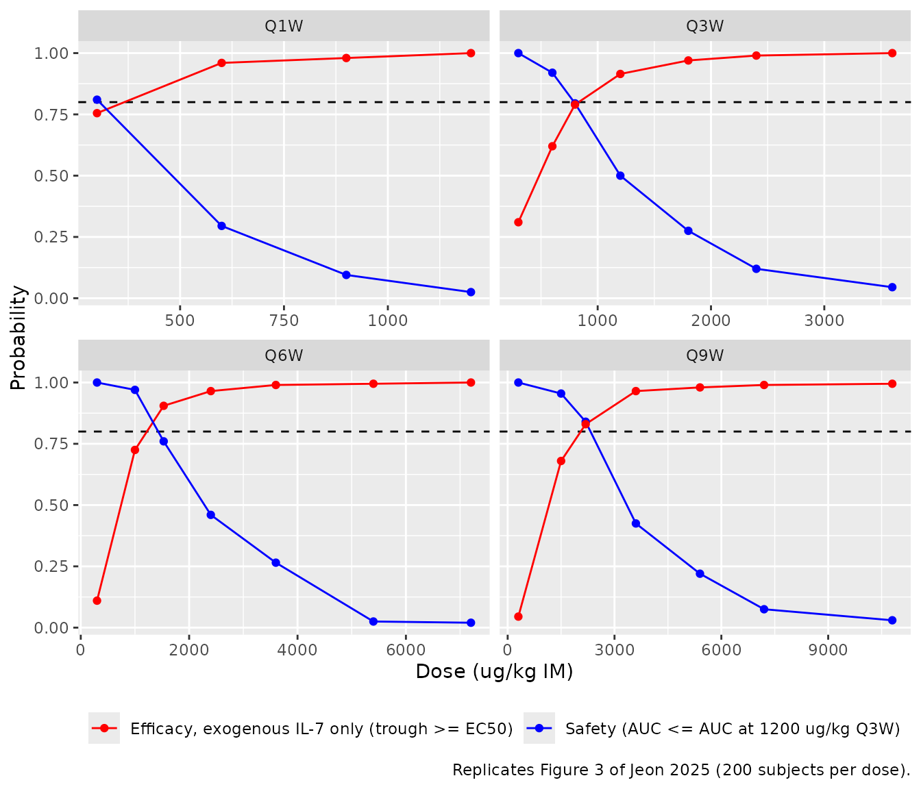

The dose at which each probability crosses 0.8 is read off by linear interpolation and compared with the published bounds:

# First change of (p >= 0.8) along the dose grid: rising for efficacy,
# falling for safety.
cross80 <- function(dose, p) {
  i <- which(diff(p >= 0.8) != 0)[1]
  if (is.na(i)) stop("probability does not cross 0.8 within the dose grid")
  dose[i] + (0.8 - p[i]) * (dose[i + 1] - dose[i]) / (p[i + 1] - p[i])
}
crossings <- prob |>
  filter(regimen != "Q1W") |>
  arrange(regimen, criterion, dose_ugkg) |>
  group_by(regimen, criterion) |>
  summarise(dose_at_0.8 = cross80(dose_ugkg, p), .groups = "drop") |>
  mutate(published = case_when(
    regimen == "Q3W" & grepl("^Safety", criterion) ~ 800,
    regimen == "Q6W" & grepl("^Safety", criterion) ~ 1530,
    regimen == "Q9W" & grepl("^Safety", criterion) ~ 2190,
    regimen == "Q3W" ~ 670,
    regimen == "Q6W" ~ 1010,
    regimen == "Q9W" ~ 1510
  ))
crossings |>
  dplyr::rename(
    "Regimen" = regimen, "Criterion" = criterion,
    "Simulated dose at P = 0.8 (ug/kg)" = dose_at_0.8,
    "Published bound (ug/kg)" = published
  ) |>
  knitr::kable(digits = 0)

Regimen	Criterion	Simulated dose at P = 0.8 (ug/kg)	Published bound (ug/kg)
Q3W	Efficacy, exogenous IL-7 only (trough >= EC50)	832	670
Q3W	Safety (AUC <= AUC at 1200 ug/kg Q3W)	792	800
Q6W	Efficacy, exogenous IL-7 only (trough >= EC50)	1221	1010
Q6W	Safety (AUC <= AUC at 1200 ug/kg Q3W)	1429	1530
Q9W	Efficacy, exogenous IL-7 only (trough >= EC50)	2052	1510
Q9W	Safety (AUC <= AUC at 1200 ug/kg Q3W)	2326	2190

safety <- crossings |> filter(grepl("^Safety", criterion))
efficacy <- crossings |> filter(grepl("^Efficacy", criterion))
q1w_safe <- prob |> filter(regimen == "Q1W", grepl("^Safety", criterion))
stopifnot(
  nrow(safety) == 3, nrow(efficacy) == 3,
  # Safety bounds: the 0.8 crossing of a 200-subject proportion moves by about
  # +/-5 % between draws (measured 742-792 / 1496-1552 / 2122-2259 ug/kg across
  # repeated cohorts); 15 % is > 3 Monte-Carlo SE and still fails if the IIV
  # on CL or Q, or the slow recycling tail, is mis-transcribed.
  all(abs(safety$dose_at_0.8 / safety$published - 1) < 0.15),
  # Efficacy: endogenous IL-7 can only add to the trough, so the exogenous-only
  # dose must be at least the published lower bound (10 % Monte-Carlo margin).
  all(efficacy$dose_at_0.8 > 0.9 * efficacy$published),
  # Q1W: the published curve is never safe. At 300 ug/kg the expected
  # proportion is ~0.70, too close to 0.8 for a 200-subject draw, so the gate
  # covers 600 ug/kg and above (expected <= 0.2).
  all(q1w_safe$p[q1w_safe$dose_ugkg >= 600] < 0.8)
)

The safety bounds are reproduced. The efficacy curve here omits each subject’s baseline IL-7, because Jeon 2025 sampled baselines from the observed mean and SD without reporting them; the exogenous-only crossings therefore sit above the published lower bounds (670, 1010 and 1510 ug/kg), by the margin that baseline IL-7 contributes to the trough.

Assumptions and deviations

• Dose units. The control stream doses pmol of rhIL-7-hyFc into the injection site with F1 = 2, annotated “AMT: GX-I7 pmol x 2 = IL7 pmol”. The maintainers read this as AMT = pmol of drug and F1 = 2 performing the doubling (dose in units$dosing). Figure 2 and the Lee 2020 Cmax values confirm it; doubling a second time would place the 20 ug/kg SC median near the observed 95th percentile.
• QSS root. The control stream computes the free concentration as 0.5 * (D + sqrt(D^2 + 4 * KSS * Ctot)). The model uses the algebraically identical rationalised root 2 * KSS * Ctot / (sqrt(D^2 + 4 * KSS * Ctot) - D). In the endosome D is about -9.2e7 pmol/L (FcRn is 92 uM), and the printed form loses precision to cancellation at low drug amounts; the structural check above confirms both roots reproduce the total.
• K_SS1. The control stream writes KSS1 = KD + Krec/KON1 with KD = 29823 hard-coded; the model computes (k_recycle + k_off1)/k_on1 (Eq. 1), whose k_off1/k_on1 = 29823.009 differs from 29823 by 3e-7 relative.
• IV dosing. F2 = 2 in the control stream is kept as f(central) = 2 for completeness; the trial had no IV arm.
• Demographics for the virtual cohorts (weight 65.3 +/- 11.1 kg) come from the primary trial report (Lee 2020), since Jeon 2025 does not tabulate them. Weight affects only the ug/kg dose.
• Figure 3 interpretation. The AUC window for the safety criterion and the definition of the trough are not stated in the paper; the choices above (18-week common window of repeated dosing; trough at the end of the first interval) are the maintainers’ and reproduce the published safety bounds. Simulations use 200 subjects per dose instead of 1000.
• Baseline IL-7 for the efficacy criterion is not reported, so the efficacy curve is exogenous-only and its lower bounds are checked one-sided.
• Covariates. None retained; age, sex, weight, height and BMI are listed in covariatesDataExcluded.
• No erratum to Jeon 2025 was found (checked 2026-10-15).