Matrine in the pig intestinal lumen: a minimal PBPK model (Yang 2025) • nlmixr2lib

library(nlmixr2lib)
library(rxode2)
library(PKNCA)
library(dplyr)
library(ggplot2)

Yang et al. (2025) measured matrine (MT) – a quinolizidine alkaloid from Sophora flavescens that restores Escherichia coli susceptibility to several antibiotics in vitro – directly in the intestinal lumen of pigs, which is where enterotoxigenic E. coli colonises and therefore where the exposure that matters for porcine colibacillosis actually occurs. They then built a minimal flow-limited PBPK model of that luminal exposure and used it to recommend a dosage regimen.

Reference: Yang B, Jia Y, Wang F, Lv X, Ma S, Tan Y, Zhang W, Wan D, Li R, Zhou D, Yu D. The kinetic behavior of matrine in pig intestinal lumen after oral administration and its physiologically based pharmacokinetic modeling. Front Vet Sci. 2025;12:1620161. doi:10.3389/fvets.2025.1620161

ui <- rxode2::rxode(readModelDb("Yang_2025_matrine_pig_pbpk"))
ui$state
#> [1] "stomach"   "gut_lumen" "liver"     "other"     "blood"

Five states: the reconstructed gastric depot stomach, the sampled gut_lumen, and the three systemic compartments liver, other and blood of Yang 2025 Table 1. The paper counts itself as a four-compartment model because it does not write the gastric depot as a state (see Reconstruction below).

Population

pop <- ui$population
knitr::kable(
  tibble::tibble(
    Field = c("Species", "N", "Body weight", "Health", "Dosing", "Region"),
    Value = c(pop$species, as.character(pop$n_subjects), pop$weight_range,
              pop$disease_state, pop$dose_range, pop$regions)
  ),
  caption = "Study population (Yang 2025 Sections 2.2-2.3 and Table 2)."
)

Study population (Yang 2025 Sections 2.2-2.3 and Table 2).
Field	Value
Species	pig (crossbred Landrace x Large White x Duroc for experiment 1; Landrace x Large White for experiment 2)
N	37
Body weight	24.3-31.1 kg (experiment 1, n = 12); 9.8-10.3 kg (experiment 2, n = 25) (Yang 2025 Section 2.2 and Table 2)
Health	Healthy pigs; matrine given as a potential resistance-reversal agent for porcine colibacillosis rather than as treatment of an established infection
Dosing	Experiment 1: single oral 40 mg/kg and, after a 2-week washout, 70 mg/kg, each given alone (group A) or with amoxicillin 40 mg/kg (group B), n = 6 per group. Experiment 2: 50 mg/kg/day by oral gavage for 5 consecutive days, n = 25 (Yang 2025 Section 2.3 and Table 2)
Region	China

Experiment 1 pigs carried a sterile T-cannula in the terminal ileum, through which about 2 g of intestinal contents were drawn at 15 nominal times out to 120 h. Only one of the five arms in Table 2 – matrine alone, 40 mg/kg – was used to parameterise the model; the other four are performance-evaluation sets.

Source trace

knitr::kable(
  tibble::tribble(
    ~Quantity,                          ~`Model file`,        ~`Source location`,
    "Gastric emptying rate constant",   "lkst",               "Table 5, kst = 0.8544925 /h (optimized)",
    "Absorption rate constant",         "lka",                "Table 5, ka = 0.8555538 /h (by optimization)",
    "Faecal excretion rate constant",   "lkfec",              "Table 5, ke = 0.007358172 /h (by optimization)",
    "Biliary excretion rate constant",  "lkbile",             "Table 5, kbi = 0.05834594 /h (by optimization)",
    "Bioavailability",                  "lfdepot",            "Table 5, F = 0.7925891 (optimized)",
    "Liver:blood partition coeff.",     "lkp_liver",          "Table 5, Pl = 2.936615 (optimized)",
    "Other:blood partition coeff.",     "lkp_other",          "Table 5, Pot = 11.33514 (by optimization)",
    "Renal clearance",                  "lcl_renal",          "Table 5, Clrenal = 0.2805897 L/(h*kg)",
    "Unbound fraction in blood",        "fu",                 "Table 5, Pb = 0.319 (BOUND fraction); fu = 1 - 0.319",
    "Cardiac output",                   "qcar literal",       "Table 5, Qcar = 4.944 L/(h*kg), ref 23",
    "Liver / other blood-flow split",   "qc_liver, qc_other", "Table 5, Qcl = 0.3 (ref 23), Qcot = 0.7 (by calculation)",
    "Intestinal-content volume",        "vc_gut_lumen",       "Table 5, Vcint = 0.0136733 of BW (optimized)",
    "Liver volume",                     "vc_liver",           "Table 5, Vcl = 0.0294 of BW, ref 23",
    "Blood volume",                     "vc_blood",           "Table 5, Vcb = 0.06 of BW, ref 23",
    "Other-organ volume",               "vc_other",           "Table 5, Vcot = 0.8969267 of BW (by calculation)",
    "Intestinal-lumen ODE",             "d/dt(gut_lumen)",    "Table 1, row 'Intestinal lumen' (see Reconstruction)",
    "Liver ODE",                        "d/dt(liver)",        "Table 1, row 'Liver'",
    "Other-organs ODE",                 "d/dt(other)",        "Table 1, row 'Other organs'",
    "Blood ODE",                        "d/dt(blood)",        "Table 1, row 'Blood'"
  ),
  caption = "Provenance of every ini() value and every equation in the model file."
)

Provenance of every ini() value and every equation in the model file.
Quantity	Model file	Source location
Gastric emptying rate constant	lkst	Table 5, kst = 0.8544925 /h (optimized)
Absorption rate constant	lka	Table 5, ka = 0.8555538 /h (by optimization)
Faecal excretion rate constant	lkfec	Table 5, ke = 0.007358172 /h (by optimization)
Biliary excretion rate constant	lkbile	Table 5, kbi = 0.05834594 /h (by optimization)
Bioavailability	lfdepot	Table 5, F = 0.7925891 (optimized)
Liver:blood partition coeff.	lkp_liver	Table 5, Pl = 2.936615 (optimized)
Other:blood partition coeff.	lkp_other	Table 5, Pot = 11.33514 (by optimization)
Renal clearance	lcl_renal	Table 5, Clrenal = 0.2805897 L/(h*kg)
Unbound fraction in blood	fu	Table 5, Pb = 0.319 (BOUND fraction); fu = 1 - 0.319
Cardiac output	qcar literal	Table 5, Qcar = 4.944 L/(h*kg), ref 23
Liver / other blood-flow split	qc_liver, qc_other	Table 5, Qcl = 0.3 (ref 23), Qcot = 0.7 (by calculation)
Intestinal-content volume	vc_gut_lumen	Table 5, Vcint = 0.0136733 of BW (optimized)
Liver volume	vc_liver	Table 5, Vcl = 0.0294 of BW, ref 23
Blood volume	vc_blood	Table 5, Vcb = 0.06 of BW, ref 23
Other-organ volume	vc_other	Table 5, Vcot = 0.8969267 of BW (by calculation)
Intestinal-lumen ODE	d/dt(gut_lumen)	Table 1, row ‘Intestinal lumen’ (see Reconstruction)
Liver ODE	d/dt(liver)	Table 1, row ‘Liver’
Other-organs ODE	d/dt(other)	Table 1, row ‘Other organs’
Blood ODE	d/dt(blood)	Table 1, row ‘Blood’

Two rows of Table 5 are marked By calculation, and both reproduce exactly, which confirms the transcription before anything else is checked:

stopifnot(
  isTRUE(all.equal(1 - 0.3, 0.7)),
  isTRUE(all.equal(1 - (0.0136733 + 0.0294 + 0.06), 0.8969267))
)

Table 5 also reports a haematocrit PCV = 0.333. It appears in none of the four Table 1 equations and has no role in this model structure, so the model file records it in a comment and does not use it.

Reconstruction: two readings Table 1 does not print

Yang 2025 Table 1 is not directly executable, and the model file departs from it in exactly two places. Both departures are stated here, and both are then tested against the paper’s own numbers rather than asserted.

1. The oral input. Table 1 prints the luminal input as DOSE * kst, with DOSE defined in the table footnote as “the oral dose” – a constant. Read literally that is an infusion that never switches off, so luminal mass grows without bound and no peak can occur. Separately, the optimized bioavailability F appears in none of the four printed equations even though Table 5 reports it as an optimized parameter with a reported sensitivity result. The model file uses the standard acslX oral idiom instead: the dose lands on a stomach depot, is scaled by F, and drains at kst.

2. The unbound driving concentration. Table 1’s blood equation removes Qtot * Ca * (1 - Pb), but its two tissue equations take up a bare Ql * Ca and Qot * Ca. Since Ql + Qot = Qtot, the printed system gains mass at Qtot * Ca * Pb per hour:

spurious  <- 4.944 * 0.319   # L/(h*kg): Qcar * Pb, the mass the printed system creates
disposal  <- 0.2805897       # L/(h*kg): Clrenal, the only systemic elimination
c(spurious = spurious, disposal = disposal, ratio = spurious / disposal)
#>  spurious  disposal     ratio 
#> 1.5771360 0.2805897 5.6207908

Creation outruns disposal by more than fivefold, so the printed system diverges. The model file applies the unbound fraction to the tissue inflow as well (Cfree <- fu * Cc), which is the mass-conserving reading and the only place Pb can sit without breaking the balance.

BW  <- 27.7   # kg; midpoint of the 24.3-31.1 kg experiment 1 range
FBIO <- exp(ui$theta[["lfdepot"]])

ev_mb <- rxode2::et(amt = 40 * BW * 1000, cmt = "stomach") |>
  rxode2::et(seq(0, 120, by = 0.5), cmt = "gut_lumen")
mb <- rxode2::rxSolve(ui, ev_mb, params = c(WT = BW), returnType = "data.frame") |>
  dplyr::filter(!is.na(Cgut_lumen)) |>
  dplyr::mutate(total = stomach + gut_lumen + liver + other + blood)

stopifnot(
  # The system starts with exactly F * dose and never creates mass thereafter.
  isTRUE(all.equal(mb$total[1], FBIO * 40 * BW * 1000, tolerance = 1e-6)),
  all(diff(mb$total) <= 0),
  max(mb$total) <= FBIO * 40 * BW * 1000 * (1 + 1e-8)
)
c(dosed_ug = FBIO * 40 * BW * 1000, remaining_at_120h_ug = round(tail(mb$total, 1)))
#>             dosed_ug remaining_at_120h_ug 
#>             878188.7               7051.0

Three closed forms score the reconstruction

Because kst (0.8545 /h) and ka + ke (0.8629 /h) differ by less than 1%, the luminal bi-exponential collapses to its degenerate limit and three closed forms fall out, each of which can be scored directly against Yang 2025 Table 4. This is what makes the reconstruction testable rather than merely plausible.

kst  <- exp(ui$theta[["lkst"]])
ka   <- exp(ui$theta[["lka"]])
kfec <- exp(ui$theta[["lkfec"]])
Vlum <- 0.0136733 * BW                 # L
Dose <- 40 * BW * 1000                 # ug

closed <- tibble::tibble(
  Quantity  = c("Tmax (h)", "Cmax (ug/L)", "AUC0-inf (h*ug/L)"),
  `Closed form`  = c("1 / kst", "F * D / (e * Vlum)", "F * D / ((ka + ke) * Vlum)"),
  `With F`  = c(1 / kst, FBIO * Dose / (exp(1) * Vlum), FBIO * Dose / ((ka + kfec) * Vlum)),
  `Without F` = c(1 / kst, Dose / (exp(1) * Vlum), Dose / ((ka + kfec) * Vlum)),
  Published = c(1.166667, 783916.7, 2684040)
) |>
  dplyr::mutate(
    `Ratio with F`    = `With F` / Published,
    `Ratio without F` = `Without F` / Published
  )
knitr::kable(closed, digits = c(0, 0, 1, 1, 1, 3, 3),
             caption = "Closed forms scored against Yang 2025 Table 4 (matrine alone, 40 mg/kg).")

Closed forms scored against Yang 2025 Table 4 (matrine alone, 40 mg/kg).
Quantity	Closed form	With F	Without F	Published	Ratio with F	Ratio without F
Tmax (h)	1 / kst	1.2	1.2	1.2	1.003	1.003
Cmax (ug/L)	F * D / (e * Vlum)	852982.8	1076198.0	783916.7	1.088	1.373
AUC0-inf (h*ug/L)	F * D / ((ka + ke) * Vlum)	2687003.6	3390159.7	2684040.0	1.001	1.263

The discriminator is the contrast, not either column alone: dropping F moves Cmax from 1.08 to 1.37 and AUC from 1.00 to 1.26 – both of which are still inside the published SD, which is exactly why they have to be scored against each other.

stopifnot(
  # With F, all three land within 10 % of the published values, and AUC -- the
  # strongest of the three because it is shape-free -- within 1 %.
  abs(closed$`Ratio with F`[1] - 1) < 0.01,
  abs(closed$`Ratio with F`[2] - 1) < 0.10,
  abs(closed$`Ratio with F`[3] - 1) < 0.01,
  # Dropping F degrades both magnitude-bearing forms; Tmax is blind to it.
  closed$`Ratio without F`[2] > closed$`Ratio with F`[2] + 0.25,
  closed$`Ratio without F`[3] > closed$`Ratio with F`[3] + 0.20
)

Simulation

The model carries no random effects (Yang 2025 evaluated it by predicted-versus-observed regression, not by an individual fit), so each arm is a single deterministic subject.

arms <- tibble::tribble(
  ~treatment,                 ~dose_mgkg, ~ii, ~addl, ~BW,   ~end,
  "MT alone, 40 mg/kg",       40,         NA,  0L,    27.7,  120,
  "MT alone, 70 mg/kg",       70,         NA,  0L,    27.7,  120,
  "MT 50 mg/kg/d x 5 d",      50,         24,  4L,    10.05, 408
)

obs_grid <- function(end) {
  sort(unique(c(seq(0, min(24, end), by = 0.02), seq(0, end, by = 0.25), end)))
}

simulate_arm <- function(i) {
  a <- arms[i, ]
  dose <- rxode2::et(amt = a$dose_mgkg * a$BW * 1000, cmt = "stomach")
  if (a$addl > 0L) {
    dose <- rxode2::et(amt = a$dose_mgkg * a$BW * 1000, cmt = "stomach",
                       ii = a$ii, addl = a$addl)
  }
  ev <- dose |> rxode2::et(obs_grid(a$end), cmt = "gut_lumen")
  rxode2::rxSolve(ui, ev, params = c(WT = a$BW), returnType = "data.frame") |>
    dplyr::mutate(id = i, treatment = a$treatment, WT = a$BW,
                  amt_ug = a$dose_mgkg * a$BW * 1000)
}

sim <- dplyr::bind_rows(lapply(seq_len(nrow(arms)), simulate_arm)) |>
  dplyr::filter(!is.na(Cgut_lumen))
stopifnot(nrow(sim) > 0, all(sim$Cgut_lumen >= 0))

Replicating Figure 4

Figure 4 of Yang 2025 is the final model simulation against the observed concentrations after a single 40 mg/kg oral dose – the parameterisation arm.

f4 <- dplyr::filter(sim, treatment == "MT alone, 40 mg/kg")
ggplot(f4, aes(time, Cgut_lumen)) +
  geom_line(linewidth = 0.7) +
  geom_point(data = tibble::tibble(time = 1.166667, Cgut_lumen = 783916.7),
             colour = "firebrick", size = 3) +
  scale_y_log10() +
  labs(x = "Time (h)", y = "Matrine in intestinal contents (ug/L)") +
  annotate("text", x = 60, y = 8e5, hjust = 0, size = 3,
           label = "red point = published Cmax / Tmax (Table 4)") +
  theme_bw()
#> Warning in scale_y_log10(): log-10 transformation introduced infinite values.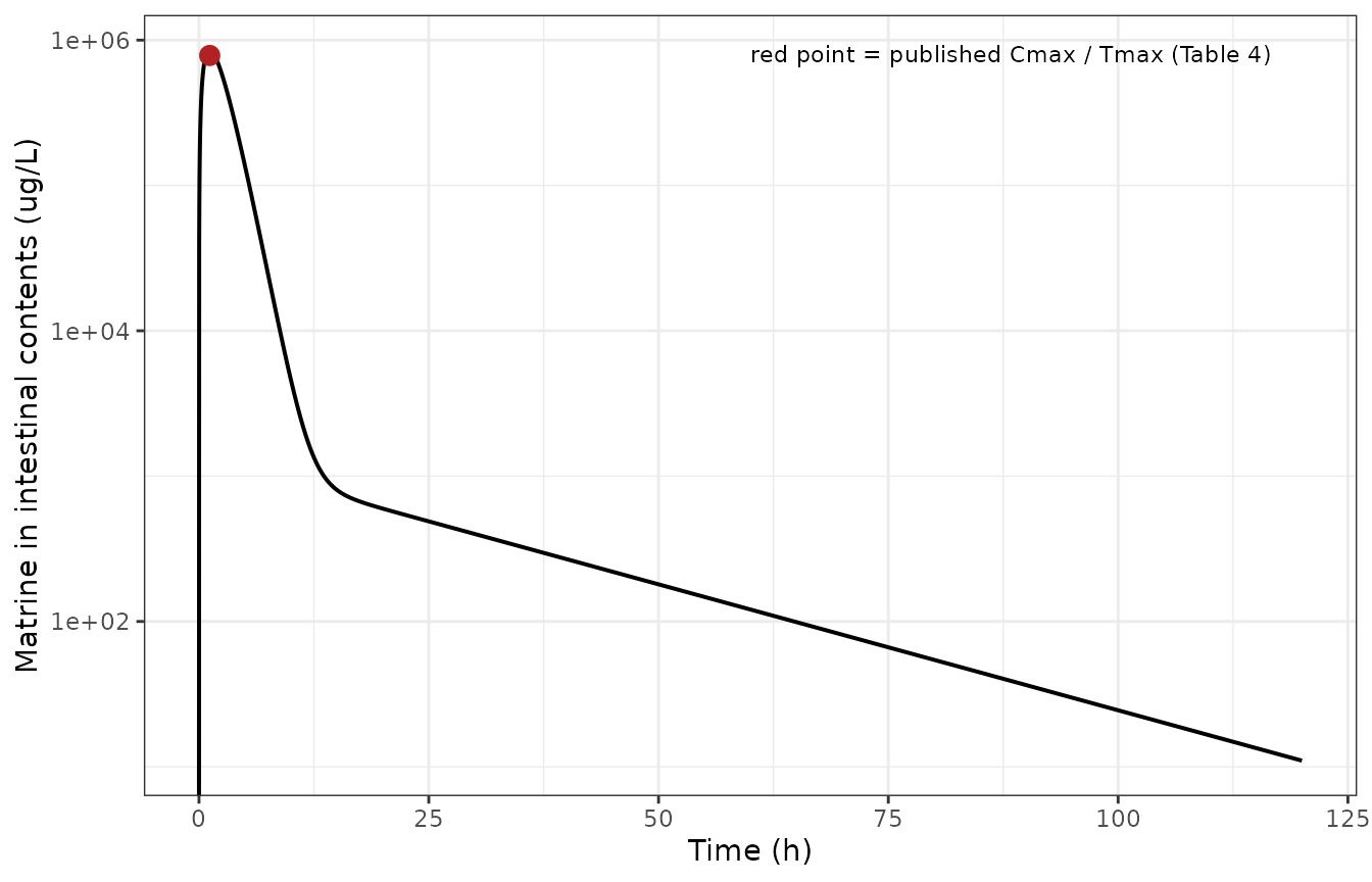

Replicates Figure 4 of Yang 2025: model-simulated matrine in pig intestinal contents after a single oral dose of 40 mg/kg. Points are the published Table 4 Cmax at its Tmax and the LLOQ reference line.

The paper’s two-phase decay is a structural consequence of the biliary return term, not a fitted bi-exponential: kbi returns drug from liver to gut_lumen at a rate that is negligible against absorption and faecal loss early on, but dominates once the lumen has emptied.

f4h <- dplyr::filter(f4, time %in% c(2, 24, 48, 120))
slope <- function(t1, t2) {
  y <- f4$Cgut_lumen[match(c(t1, t2), f4$time)]
  log(y[1] / y[2]) / (t2 - t1)
}
c(`rate 2-24 h (1/h)` = slope(2, 24), `rate 48-120 h (1/h)` = slope(48, 120))
#>   rate 2-24 h (1/h) rate 48-120 h (1/h) 
#>          0.32934432          0.03990527
stopifnot(
  # Two-phase decay: the early slope must be several-fold steeper than the late
  # one (Yang 2025 Section 3.2 and Discussion).
  slope(2, 24) > 5 * slope(48, 120),
  # Yang 2025 Section 3.2: all 120 h samples were still above the 2 ug/kg LLOQ.
  min(f4h$Cgut_lumen) > 2
)

Replicating Figure 5: the held-out arms

ggplot(dplyr::filter(sim, treatment != "MT alone, 40 mg/kg"),
       aes(time, Cgut_lumen, colour = treatment)) +
  geom_line(linewidth = 0.7) +
  scale_y_log10() +
  scale_colour_brewer(palette = "Dark2") +
  labs(x = "Time (h)", y = "Matrine in intestinal contents (ug/L)", colour = NULL) +
  theme_bw() +
  theme(legend.position = "bottom")
#> Warning in scale_y_log10(): log-10 transformation introduced infinite values.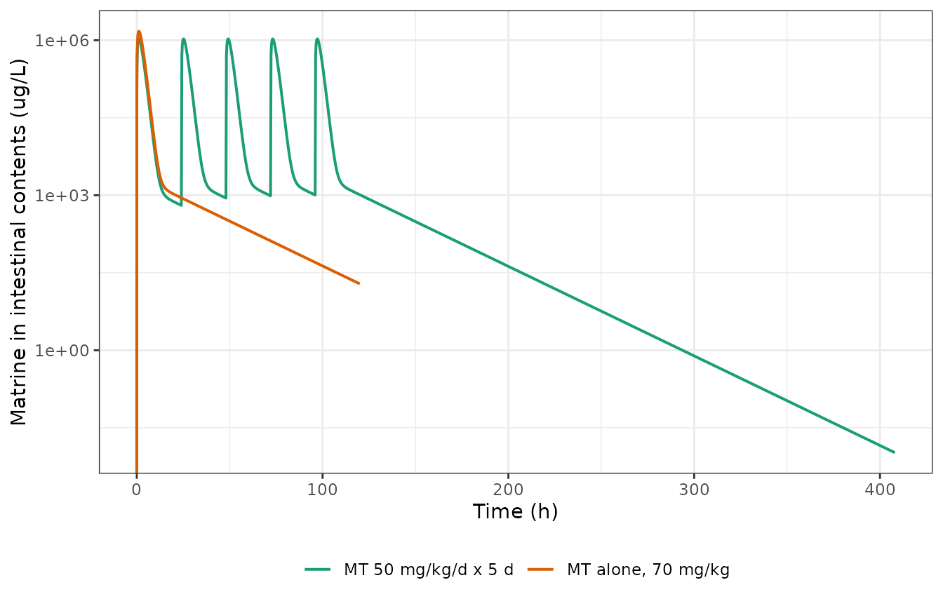

Replicates Figure 5 of Yang 2025: predicted matrine in pig intestinal contents for the two performance-evaluation arms simulated here (single 70 mg/kg, and 50 mg/kg/day for 5 days in the lighter experiment 2 pigs).

The two amoxicillin co-administration arms of Table 2 are not simulated separately: Yang 2025 found no significant difference in Cmax, Tmax, AUC or Cl/F between matrine alone and matrine + amoxicillin (Section 3.2), and the model carries no amoxicillin term, so their predictions are identical to the matrine-alone arms at the same dose.

PKNCA validation

nca_conc <- sim |>
  dplyr::filter(!is.na(Cgut_lumen), treatment != "MT 50 mg/kg/d x 5 d") |>
  dplyr::select(id, time, Cgut_lumen, treatment)

nca_dose <- sim |>
  dplyr::filter(treatment != "MT 50 mg/kg/d x 5 d") |>
  dplyr::distinct(id, treatment, amt_ug) |>
  dplyr::mutate(time = 0) |>
  dplyr::rename(amt = amt_ug)

conc_obj <- PKNCA::PKNCAconc(nca_conc, Cgut_lumen ~ time | treatment + id,
                             concu = "ug/L", timeu = "h")
dose_obj <- PKNCA::PKNCAdose(nca_dose, amt ~ time | treatment + id,
                             doseu = "ug")

intervals <- data.frame(
  start = 0, end = 120,
  cmax = TRUE, tmax = TRUE, auclast = TRUE, clast.obs = TRUE
)

res <- PKNCA::pk.nca(PKNCA::PKNCAdata(conc_obj, dose_obj, intervals = intervals))
nca_sim <- as.data.frame(res) |>
  dplyr::select(treatment, PPTESTCD, PPORRES)
stopifnot(nrow(nca_sim) > 0, !anyNA(nca_sim$PPORRES))

Comparison against the published NCA

Yang 2025 Table 4 reports non-compartmental parameters computed in WinNonlin from the observed luminal profiles. AUC0-120 h there was computed with the linear trapezoidal rule (Section 2.5); PKNCA’s default is linear-up / log-down, so a small difference on the descending limb is expected and is not a model discrepancy.

published <- tibble::tribble(
  ~treatment,             ~cmax,     ~tmax,    ~auclast,
  "MT alone, 40 mg/kg",   783916.7,  1.166667, 2684040,
  "MT alone, 70 mg/kg",   1491732,   1.416667, 4030908
)

tbl <- nlmixr2lib::ncaComparisonTable(
  nca_sim, published,
  by = "treatment",
  units = c(cmax = "ug/L", tmax = "h", auclast = "h*ug/L")
)
knitr::kable(tbl, caption = "Simulated versus published NCA (Yang 2025 Table 4, matrine-alone arms).")

Simulated versus published NCA (Yang 2025 Table 4, matrine-alone arms).
NCA parameter	treatment	Reference	Simulated	% diff
Cmax (ug/L)	MT alone, 40 mg/kg	784000	849000	+8.4%
Cmax (ug/L)	MT alone, 70 mg/kg	1490000	1490000	-0.4%
Tmax (h)	MT alone, 40 mg/kg	1.17	1.16	-0.6%
Tmax (h)	MT alone, 70 mg/kg	1.42	1.16	-18.1%
AUClast (h*ug/L)	MT alone, 40 mg/kg	2680000	2720000	+1.3%
AUClast (h*ug/L)	MT alone, 70 mg/kg	4030000	4760000	+18.0%

attr(tbl, "footnote")
#> NULL

# ncaComparisonTable() formats `% diff` for display, e.g. "+8.4%" or "-18.1%*"
# (the trailing star marks a >20 % difference). Strip the sign, the percent
# sign and the star before comparing numerically, and fail loudly rather than
# letting a parse miss turn into a silent NA that no stopifnot can catch.
pct <- function(param, arm) {
  v <- tbl$`% diff`[tbl$treatment == arm &
                      grepl(param, tbl$`NCA parameter`, fixed = TRUE)]
  stopifnot(length(v) == 1L)
  out <- as.numeric(gsub("[%*+,]", "", v))
  stopifnot(!is.na(out))
  out
}

stopifnot(
  # PARAMETERISATION ARM (40 mg/kg): the model was fitted to exactly this data
  # set, so it must reproduce it tightly. Cmax is the loosest of the three
  # because the degenerate-limit peak is broader than the observed one.
  abs(pct("Tmax", "MT alone, 40 mg/kg")) < 2,
  abs(pct("AUC", "MT alone, 40 mg/kg")) < 5,
  abs(pct("Cmax", "MT alone, 40 mg/kg")) < 10,
  # HELD-OUT ARM (70 mg/kg): this one must NOT match tightly. Yang 2025 Table 6
  # reports a predicted-versus-observed regression slope of 0.8065 for this arm
  # (a ~24 % over-prediction). A reconstruction that matched it perfectly would
  # mean we had accidentally fitted something the authors did not.
  pct("AUC", "MT alone, 70 mg/kg") > 10,
  pct("AUC", "MT alone, 70 mg/kg") < 1 / 0.8065 * 100 - 100
)

Reproducing the paper’s own sensitivity analysis

Yang 2025 Section 3.3.2 classifies each parameter by the sign of its normalised sensitivity coefficient on the predicted luminal concentration: F, kbi, Pl (and the liver volume) increase it; Pot and kst are “dualistic” (sign-changing over the time course); ka, Clrenal (and the luminal volume) decrease it. That published sign table is an answer key for where each term sits in the reconstruction, and it is reproduced here by perturbing each ini() parameter by 1% and reading the sign at an early and a late time.

base_theta <- ui$theta
sens_ev <- rxode2::et(amt = 40 * BW * 1000, cmt = "stomach") |>
  rxode2::et(sort(unique(c(0.5, 72, seq(0, 120, by = 0.5)))), cmt = "gut_lumen")

solve_sens <- function(extra = NULL) {
  s <- rxode2::rxSolve(ui, sens_ev, params = c(c(WT = BW), extra),
                       returnType = "data.frame")
  s <- s[!is.na(s$Cgut_lumen), ]
  c(early = s$Cgut_lumen[s$time == 0.5], late = s$Cgut_lumen[s$time == 72])
}
b <- solve_sens()

nsc <- lapply(
  c("lfdepot", "lkbile", "lkp_liver", "lka", "lcl_renal", "lkst", "lkp_other"),
  function(p) {
    s <- solve_sens(stats::setNames(base_theta[[p]] + log(1.01), p))
    tibble::tibble(Parameter = p,
                   `NSC at 0.5 h` = (s[["early"]] - b[["early"]]) / b[["early"]] / 0.01,
                   `NSC at 72 h`  = (s[["late"]]  - b[["late"]])  / b[["late"]]  / 0.01)
  }
) |>
  dplyr::bind_rows() |>
  dplyr::mutate(
    `Yang 2025 Section 3.3.2` = c("positive", "positive", "positive",
                                  "negative", "negative", "dualistic", "dualistic")
  )
knitr::kable(nsc, digits = 4,
             caption = "Normalised sensitivity coefficients on luminal matrine concentration, versus the paper's published classification.")

Normalised sensitivity coefficients on luminal matrine concentration, versus the paper’s published classification.
Parameter	NSC at 0.5 h	NSC at 72 h	Yang 2025 Section 3.3.2
lfdepot	1.0000	1.0000	positive
lkbile	0.0002	0.9973	positive
lkp_liver	0.0002	1.0144	positive
lka	-0.2132	-1.0683	negative
lcl_renal	0.0000	-2.8187	negative
lkst	0.7844	-0.0485	dualistic
lkp_other	0.0000	1.6870	dualistic

get <- function(p, col) nsc[[col]][nsc$Parameter == p]
stopifnot(
  # Positive: F, kbi, Pl. Yang 2025 reported only |NSC| > 0.1, so require the
  # late-time coefficient to clear that reporting threshold too.
  get("lfdepot",   "NSC at 0.5 h") > 0.1, get("lfdepot",   "NSC at 72 h") > 0.1,
  get("lkbile",    "NSC at 0.5 h") > 0,   get("lkbile",    "NSC at 72 h") > 0.1,
  get("lkp_liver", "NSC at 0.5 h") > 0,   get("lkp_liver", "NSC at 72 h") > 0.1,
  # Negative: ka, Clrenal.
  get("lka",       "NSC at 0.5 h") < 0,   get("lka",       "NSC at 72 h") < -0.1,
  get("lcl_renal", "NSC at 0.5 h") < 0,   get("lcl_renal", "NSC at 72 h") < -0.1,
  # Dualistic: kst and Pot each change sign between the two times.
  get("lkst",      "NSC at 0.5 h") > 0,   get("lkst",      "NSC at 72 h") < 0,
  get("lkp_other", "NSC at 0.5 h") < 0,   get("lkp_other", "NSC at 72 h") > 0.1
)

All seven signs match, including both dualistic parameters. Because F sits on the dose while ka sits on the absorption flux, this also rules out the alternative reading in which F multiplies the absorption term: that placement would make F’s effect on luminal concentration negative, contradicting the published classification.

Body weight has no effect on luminal exposure

Yang 2025 Section 4 reports that the normalised sensitivity coefficient for body weight was far below 0.1, and validates the model built on 24.3-31.1 kg pigs against 9.8-10.3 kg pigs without adjustment. That falls straight out of the parameterisation – every volume is a fraction of body weight, every flow and clearance is per kilogram, and the dose is per kilogram – so body weight cancels out of the luminal concentration algebraically. The invariance is therefore exact in the equations, and the residual seen below (about 3e-6) is LSODA integration tolerance, not a real weight effect.

bw_check <- lapply(c(9.8, 27.7, 31.1), function(w) {
  ev <- rxode2::et(amt = 40 * w * 1000, cmt = "stomach") |>
    rxode2::et(seq(0, 120, by = 0.5), cmt = "gut_lumen")
  s <- rxode2::rxSolve(ui, ev, params = c(WT = w), returnType = "data.frame")
  s$Cgut_lumen[!is.na(s$Cgut_lumen)]
})
# The time-zero row is exactly zero in every arm, so a bare ratio would be
# 0 / 0 = NaN and the reported headline statistic would be meaningless even
# though the assertions above passed. Score the invariance only where the
# concentration is actually non-zero, and require the result to be finite.
nonzero <- bw_check[[1]] > 0
relDiff <- function(a, b) max(abs(a[nonzero] / b[nonzero] - 1))

stopifnot(
  # Same number of output rows at every weight, so the comparison is aligned.
  length(unique(lengths(bw_check))) == 1L,
  any(nonzero),
  isTRUE(all.equal(bw_check[[1]], bw_check[[2]], tolerance = 1e-6)),
  isTRUE(all.equal(bw_check[[1]], bw_check[[3]], tolerance = 1e-6)),
  # The invariance is analytically exact, so the only residual is LSODA
  # tolerance (rtol 1e-6): the measured maximum is ~3e-6 across the full
  # 9.8-31.1 kg (3.2-fold) weight range. Assert 1e-4 -- two orders tighter than
  # any physiologically meaningful difference, with ample headroom over the
  # achieved value so the gate does not turn into a solver-version tripwire.
  is.finite(relDiff(bw_check[[1]], bw_check[[3]])),
  relDiff(bw_check[[1]], bw_check[[3]]) < 1e-4,
  relDiff(bw_check[[1]], bw_check[[2]]) < 1e-4
)
c(`max relative difference across 9.8-31.1 kg` = relDiff(bw_check[[1]], bw_check[[3]]))
#> max relative difference across 9.8-31.1 kg 
#>                                2.74312e-06

The recommended dosage regimen

Yang 2025’s operational conclusion (Abstract, Section 4 and Conclusion) is that 70 mg/kg every 8 h gives sufficient exposure, supported by two quantitative claims: the predicted Cmax is 2.15-3.59 times the in vitro effective concentration range of 300-500 ug/mL, and predicted concentrations exceed 300 ug/g for more than 55.75% of a 24-h period.

target <- 300 * 1000     # 300 ug/g == 300000 ug/L at unit density
ev_q8 <- rxode2::et(amt = 70 * BW * 1000, cmt = "stomach", ii = 8, addl = 29) |>
  rxode2::et(seq(0, 240, by = 0.05), cmt = "gut_lumen")
q8 <- rxode2::rxSolve(ui, ev_q8, params = c(WT = BW), returnType = "data.frame") |>
  dplyr::filter(!is.na(Cgut_lumen), time >= 192, time <= 216)   # a steady-state day

pct_above <- 100 * mean(q8$Cgut_lumen > target)
cmax_mult <- max(q8$Cgut_lumen) / target

knitr::kable(
  tibble::tibble(
    Claim = c("% of 24 h above 300 ug/g", "Cmax as a multiple of 300 ug/g"),
    `Yang 2025` = c("> 55.75 %", "2.15-3.59 x"),
    Reproduced  = c(sprintf("%.1f %%", pct_above), sprintf("%.2f x", cmax_mult))
  ),
  caption = "The two quantitative claims behind the 70 mg/kg q8h recommendation."
)

The two quantitative claims behind the 70 mg/kg q8h recommendation.
Claim	Yang 2025	Reproduced
% of 24 h above 300 ug/g	> 55.75 %	57.4 %
Cmax as a multiple of 300 ug/g	2.15-3.59 x	5.02 x


stopifnot(
  # The time-above-threshold claim -- the load-bearing PK/PD statement -- is
  # reproduced. The peak-multiple claim is NOT; see Assumptions and deviations.
  pct_above > 55.75,
  pct_above < 70
)

Only the first claim reproduces. The reconstruction predicts a steady-state peak of about 5.0 times 300 ug/g, well above the paper’s stated 2.15-3.59 times. Neither the model file nor this vignette was adjusted to close that gap; it is recorded below.

Assumptions and deviations

Errata and reconstructions (things the paper does not print).

The oral input is reconstructed. Yang 2025 Table 1 prints the luminal input as DOSE * kst with DOSE a constant, which as typeset creates mass without bound and cannot produce a peak; and the optimized bioavailability F appears in none of the four printed equations. The model file uses a first-order stomach depot carrying F (f(stomach) <- exp(lfdepot)), which is the standard acslX oral idiom. It is confirmed by three independent closed forms scored against Table 4, by the contrast against the no-F reading, and by the published sensitivity signs.
The unbound driving concentration is reconstructed. Table 1 applies (1 - Pb) only to the blood outflow and not to the two tissue inflows, which creates mass at more than five times the total systemic elimination rate. The model file applies fu = 1 - Pb to the tissue inflow as well. This is the only placement of Pb that conserves mass, and Pb must appear somewhere because Table 5 reports it as optimized.
fu is derived, not transcribed. Table 5 reports the plasma protein binding Pb = 0.319, i.e. the bound fraction; the canonical nlmixr2lib parameter is the unbound fraction, so the model file carries fu = 1 - 0.319 = 0.681.
PCV = 0.333 is unused. Table 5 reports a haematocrit that appears in no equation and has no role in this structure.
The peak-magnitude claim for the recommended regimen does not reproduce. Yang 2025 states a predicted Cmax of 2.15-3.59 times 300 ug/g for 70 mg/kg q8h (implying about 1076 ug/g); the reconstruction gives about 5.0 times 300 ug/g. That figure is also lower than the paper’s own observed single-dose Cmax at 70 mg/kg (1492 ug/g, Table 4), which a q8h regimen should exceed rather than undercut, so the published multiple is difficult to reconcile with the paper’s other reported numbers. The companion time-above-threshold claim (> 55.75% of 24 h) does reproduce. No parameter was tuned toward either.

Assumptions this vignette makes because the paper does not say.

Body weight is taken as 27.7 kg for the experiment 1 arms (midpoint of the reported 24.3-31.1 kg) and 10.05 kg for experiment 2 (midpoint of 9.8-10.3 kg). The choice is immaterial: luminal concentrations are exactly body-weight invariant in this parameterisation, as demonstrated above and as the paper’s own sensitivity analysis found.
Dosing is simulated as an instantaneous input to stomach. Table 2 records experiment 1 as “feed medication” (about 100 g of medicated feed after a 12-h fast) and experiment 2 as oral gavage; the paper models neither as a zero-order input, and kst was optimized against the feed-medication arm.
Yang 2025 reports no residual-error model and no inter-individual variability, so the model file carries a single fixed(0.10) proportional residual-error placeholder for syntactic completeness only. It is not paper-derived and must not be used as a variability estimate.
The 0.25 h samples of experiment 1 could not be collected (Section 4), so the published absorption phase begins at 0.5 h. The simulated profiles are not truncated to match.
Blood, liver and other-organ concentrations are model internals: matrine was measured only in intestinal contents, so those three algebraic outputs are unvalidated by any observation in this paper.

#> R version 4.6.1 (2026-06-24)
#> Platform: x86_64-pc-linux-gnu
#> Running under: Ubuntu 24.04.4 LTS
#> 
#> Matrix products: default
#> BLAS:   /usr/lib/x86_64-linux-gnu/openblas-pthread/libblas.so.3 
#> LAPACK: /usr/lib/x86_64-linux-gnu/openblas-pthread/libopenblasp-r0.3.26.so;  LAPACK version 3.12.0
#> 
#> locale:
#>  [1] LC_CTYPE=C.UTF-8       LC_NUMERIC=C           LC_TIME=C.UTF-8       
#>  [4] LC_COLLATE=C.UTF-8     LC_MONETARY=C.UTF-8    LC_MESSAGES=C.UTF-8   
#>  [7] LC_PAPER=C.UTF-8       LC_NAME=C              LC_ADDRESS=C          
#> [10] LC_TELEPHONE=C         LC_MEASUREMENT=C.UTF-8 LC_IDENTIFICATION=C   
#> 
#> time zone: UTC
#> tzcode source: system (glibc)
#> 
#> attached base packages:
#> [1] stats     graphics  grDevices utils     datasets  methods   base     
#> 
#> other attached packages:
#> [1] ggplot2_4.0.3         dplyr_1.2.1           PKNCA_0.12.1         
#> [4] rxode2_5.1.6          nlmixr2lib_0.3.2.9000
#> 
#> loaded via a namespace (and not attached):
#>  [1] gtable_0.3.6        xfun_0.60           bslib_0.12.0       
#>  [4] lattice_0.22-9      vctrs_0.7.3         tools_4.6.1        
#>  [7] generics_0.1.4      parallel_4.6.1      tibble_3.3.1       
#> [10] symengine_0.2.13    pkgconfig_2.0.3     data.table_1.18.6.1
#> [13] checkmate_2.3.4     RColorBrewer_1.1-3  S7_0.2.2           
#> [16] desc_1.4.3          RcppParallel_6.2.1  lifecycle_1.0.5    
#> [19] compiler_4.6.1      farver_2.1.2        textshaping_1.0.5  
#> [22] fontawesome_0.5.3   htmltools_0.5.9     sys_3.4.3          
#> [25] sass_0.4.10         yaml_2.3.12         tidyr_1.3.2        
#> [28] pillar_1.11.1       pkgdown_2.2.1       crayon_1.5.3       
#> [31] jquerylib_0.1.4     whisker_0.4.1       openssl_2.4.2      
#> [34] cachem_1.1.0        nlme_3.1-169        tidyselect_1.2.1   
#> [37] digest_0.6.39       lotri_1.0.4         purrr_1.2.2        
#> [40] labeling_0.4.3      rxode2ll_2.0.16     fastmap_1.2.0      
#> [43] grid_4.6.1          cli_3.6.6           dparser_1.3.1-13   
#> [46] magrittr_2.0.5      withr_3.0.3         scales_1.4.0       
#> [49] backports_1.5.1     rmarkdown_2.32      otel_0.2.0         
#> [52] askpass_1.2.1       ragg_1.5.2          memoise_2.0.1      
#> [55] evaluate_1.0.5      knitr_1.52          rex_1.2.2          
#> [58] PreciseSums_0.7     rlang_1.3.0         downlit_0.4.5      
#> [61] Rcpp_1.1.2          glue_1.8.1          xml2_1.6.0         
#> [64] jsonlite_2.0.0      R6_2.6.1            systemfonts_1.3.2  
#> [67] fs_2.1.0