Pioglitazone in MASH: liver histology and transaminases (Tran 2026)
Source:vignettes/articles/Tran_2026_pioglitazone_mash.Rmd
Tran_2026_pioglitazone_mash.RmdModel and source
Tran et al. (2026) report a model-based meta-analysis (MBMA) of pioglitazone in metabolic dysfunction-associated steatohepatitis (MASH, formerly NASH). The paper fits six separate models, and each is a separate file in nlmixr2lib:
| Model | Endpoint | Form |
|---|---|---|
Tran_2026_pioglitazone_steatosis_mbma |
steatosis grade 0-3 | proportional odds,
alpha * log(dose) * t / (ET50 + t)
|
Tran_2026_pioglitazone_inflammation_mbma |
lobular inflammation grade 0-3 | proportional odds, alpha * log(dose)
|
Tran_2026_pioglitazone_ballooning_mbma |
hepatocyte ballooning grade 0-2 | proportional odds, alpha * dose * t / (ET50 + t)
|
Tran_2026_pioglitazone_fibrosis_mbma |
fibrosis stage 0-4 | proportional odds, alpha * log(dose)
|
Tran_2026_pioglitazone_alt_mbma |
arm-mean ALT (U/L) | Weibull decline to a plateau |
Tran_2026_pioglitazone_ast_mbma |
arm-mean AST (U/L) | Weibull decline to a plateau |
- Citation: Tran QT, Bui TT, Ngo LT, Yang BR, Baek IH, Nguyen VH, Lee KA, Yun HY, Chae JW, Lee S, Kim JH, Jung W. Model-Based Meta-Analysis of the Relationship Between Pioglitazone and Histological Outcomes in Metabolic Dysfunction-Associated Steatohepatitis Patients. CPT Pharmacometrics Syst Pharmacol. 2026;15:e70034. doi:10.1002/psp4.70034.
- Article: https://doi.org/10.1002/psp4.70034 (open access; PMC12823776)
# Two expected rxSolve() warnings are muffled, and only those: the ordinal
# histology models carry no residual-error parameter ("No sigma parameters in
# the model"), and typical-value solves of several subjects run with the random
# effects removed ("multi-subject simulation without ... 'omega'").
solve_quiet <- function(ui, data) {
  withCallingHandlers(
    rxode2::rxSolve(ui, data),
    warning = function(w) {
      if (grepl("No sigma parameters|multi-subject simulation without", conditionMessage(w))) {
        invokeRestart("muffleWarning")
      }
    }
  )
}

endpoints <- c("steatosis", "inflammation", "ballooning", "fibrosis")
hist_ui <- lapply(
  setNames(endpoints, endpoints),
  function(e) rxode2::rxode(readModelDb(sprintf("Tran_2026_pioglitazone_%s_mbma", e)))
)
alt_ui <- rxode2::rxode(readModelDb("Tran_2026_pioglitazone_alt_mbma"))
ast_ui <- rxode2::rxode(readModelDb("Tran_2026_pioglitazone_ast_mbma"))
Population
Eight trials with 540 patients in total were included (Tran 2026 Results 3.1; Table S2): Aithal 2008, Belfort 2006, Cusi 2016, Huang 2021, Lutchman 2007, Promrat 2006, Sanyal 2010 and Sharma 2012. All enrolled adults with biopsy-proven NASH. Arm mean ages ranged from 40.4 to 55 years, and some trials enrolled patients with type 2 diabetes or prediabetes. Pioglitazone was given at 30 or 45 mg/day for 6 to 24 months; Belfort 2006 and Cusi 2016 started at 30 mg/day and increased to 45 mg/day after 2 months. Sex, weight and race were not tabulated.
The histology endpoints were reported only before and after treatment, as counts per grade or as a mean and SD. The authors turned each arm and time into 500 virtual patients, by bootstrap resampling of the counts or from a beta distribution matched to the mean and SD, and fitted the ordinal models to those virtual patients (Methods 2.2.1 and the supplementary code). Five trials contributed steatosis data, four inflammation, five ballooning and all eight fibrosis (Table S3). ALT and AST were modelled as arm means over time from eight and seven trials (Figure S2).
str(hist_ui$steatosis$population)
#> List of 11
#>  $ species       : chr "human"
#>  $ n_subjects    : int 540
#>  $ n_studies     : int 8
#>  $ age_range     : chr "arm mean ages 40.4-55 years (Tran 2026 Table S2)"
#>  $ weight_range  : chr "not reported"
#>  $ sex_female_pct: num NA
#>  $ race_ethnicity: chr "not reported"
#>  $ disease_state : chr "biopsy-proven metabolic dysfunction-associated steatohepatitis (MASH, formerly NASH), with or without type 2 di"| __truncated__
#>  $ dose_range    : chr "pioglitazone 30 or 45 mg/day orally (Belfort 2006 and Cusi 2016 started at 30 mg/day and increased to 45 mg/day"| __truncated__
#>  $ regions       : chr "not reported at study level"
#>  $ notes         : chr "Steatosis model: five of the eight trials contributed steatosis data (Belfort 2006, Cusi 2016, Huang 2021, Sany"| __truncated__
Source trace
Every value is from Tran 2026 Table 1 (histology) or Table 2 (liver enzymes); the equations are from Methods 2.2.1 and 2.2.2 and the Table 2 footnote.
| Model | Parameter | Value | Source |
|---|---|---|---|
| all four histology models | logit P(Y <= m) = sum_{L=0}^{m} beta_L + f(dose, time) + eta |
– | Methods 2.2.1 |
| steatosis |
logite0 (beta_0) |
-3.07 | Table 1 |
| steatosis |
logitstep1, logitstep2 (beta_1,
beta_2) |
2.12, 1.31 | Table 1 |
| steatosis |
e_dose_pio_mgd_steatosis (alpha, on log(dose)) |
0.49 | Table 1; Results 3.2.1 |
| steatosis | ET50 (let50) |
0.584 month | Table 1 (‘EC50 (month)’) |
| steatosis |
etalogite0,
etae_dose_pio_mgd_steatosis
|
0.0298, 0.244 | Table 1 OMEGA |
| inflammation |
logite0, logitstep1,
logitstep2
|
-2.44, 2.58, 3.06 | Table 1 |
| inflammation |
e_dose_pio_mgd_inflammation (alpha, on log(dose)) |
0.413 | Table 1 |
| inflammation |
etalogite0,
etae_dose_pio_mgd_inflammation
|
0.35, 0.329 | Table 1 OMEGA |
| ballooning |
logite0, logitstep1
|
-1.12, 1.7 | Table 1 |
| ballooning |
e_dose_pio_mgd_ballooning (alpha, on dose) |
0.0835 per mg/day | Table 1; Results 3.2.1 (dOFV = 56) |
| ballooning | ET50 (let50) |
17.4 month | Table 1 (‘EC50 (month)’) |
| ballooning | etalogite0 |
0.232 | Table 1 OMEGA |
| fibrosis |
logite0, logitstep1 to
logitstep3
|
-0.946, 1.36, 0.946, 1.28 | Table 1 |
| fibrosis |
e_dose_pio_mgd_fibrosis (alpha, on log(dose)) |
0.168 | Table 1 |
| fibrosis | etalogite0 |
0.086 | Table 1 OMEGA |
| ALT, AST | Effect = Baseline + A * exp(-lambda * time^gamma) |
– | Methods 2.2.2; Table 2 footnote |
| ALT |
rmin_alt (Baseline), wamp_alt (A) |
33.9, 39.1 U/L | Table 2 |
| ALT |
wlambda_placebo, wlambda_drug (lambda1,
lambda2) |
0.0689, 0.534 | Table 2 |
| ALT | wgamma |
0.703 | Table 2 |
| ALT |
eta_study_lrmin_alt,
eta_study_lwamp_alt
|
0.0332, 0.157 | Table 2 Omega |
| ALT |
propSd, addSd
|
0.292, 10.5 U/L | Table 2 |
| AST |
rmin_ast (Baseline), wamp_ast (A) |
29.6, 16.1 U/L | Table 2 |
| AST |
wlambda_placebo, wlambda_drug
|
0.0352, 0.694 | Table 2 |
| AST | wgamma |
0.591 | Table 2 |
| AST |
eta_study_lrmin_ast,
eta_study_lwamp_ast
|
0.0072, 0.0782 | Table 2 Omega |
| AST |
propSd (additive fixed to 0) |
0.352 | Table 2 |
Histology: proportional-odds models
Structure check against the closed form
With the random effects at zero, each model’s per-grade probabilities
must equal the inverse logit of the running sums of Table 1. This checks
the threshold indexing, the natural log of the dose and the
t / (ET50 + t) term in one step. Both sides use the same
parameters, so the bound is tight.
grid <- expand.grid(time = c(0, 1, 6, 18, 24), DOSE_PIO_MGD = c(0, 30, 45))
grid <- grid[!(grid$time == 0 & grid$DOSE_PIO_MGD > 0), ]
grid$id <- seq_len(nrow(grid))
grid$evid <- 0

# Table 1: thresholds (beta_0, beta_1, ...), alpha, dose form, ET50.
table1 <- list(
  steatosis = list(beta = c(-3.07, 2.12, 1.31), alpha = 0.49, f = "log", et50 = 0.584),
  inflammation = list(beta = c(-2.44, 2.58, 3.06), alpha = 0.413, f = "log", et50 = NA),
  ballooning = list(beta = c(-1.12, 1.7), alpha = 0.0835, f = "linear", et50 = 17.4),
  fibrosis = list(beta = c(-0.946, 1.36, 0.946, 1.28), alpha = 0.168, f = "log", et50 = NA)
)

closed_form <- function(p, dose, time) {
  fdose <- if (p$f == "log") ifelse(dose > 0, log(pmax(dose, 1)), 0) else dose
  ftime <- if (is.na(p$et50)) 1 else time / (p$et50 + time)
  lp <- outer(p$alpha * fdose * ftime, cumsum(p$beta), "+")
  cum <- cbind(plogis(lp), 1)
  cbind(cum[, 1], t(apply(cum, 1, diff)))
}

for (e in endpoints) {
  sim <- as.data.frame(solve_quiet(rxode2::zeroRe(hist_ui[[e]]), grid))
  pcols <- paste0("p", 0:length(table1[[e]]$beta))
  ref <- closed_form(table1[[e]], grid$DOSE_PIO_MGD, grid$time)
  stopifnot(
    all(abs(as.matrix(sim[, pcols]) - ref) < 1e-10),
    all(abs(rowSums(sim[, pcols]) - 1) < 1e-10)
  )
}
Typical (random effects at zero) grade distributions without drug and after 18 months of pioglitazone:
typical <- bind_rows(lapply(endpoints, function(e) {
  sim <- as.data.frame(solve_quiet(rxode2::zeroRe(hist_ui[[e]]), grid))
  sim |>
    filter(time %in% c(0, 18)) |>
    select(time, DOSE_PIO_MGD, starts_with("p")) |>
    select(-starts_with("pcum")) |>
    mutate(endpoint = e)
})) |>
  pivot_longer(starts_with("p"), names_to = "grade", values_to = "prob") |>
  filter(!is.na(prob)) |>
  mutate(grade = sub("^p", "", grade))

typical |>
  mutate(regimen = case_when(
    time == 0 ~ "pre-treatment",
    DOSE_PIO_MGD == 0 ~ sprintf("placebo, month %d", time),
    TRUE ~ sprintf("%d mg/day, month %d", DOSE_PIO_MGD, time)
  )) |>
  select(endpoint, regimen, grade, prob) |>
  pivot_wider(names_from = grade, values_from = prob, names_prefix = "grade ") |>
knitr::kable(digits = 3)| endpoint | regimen | grade 0 | grade 1 | grade 2 | grade 3 | grade 4 |
|---|---|---|---|---|---|---|
| steatosis | pre-treatment | 0.044 | 0.235 | 0.310 | 0.411 | |
| steatosis | placebo, month 18 | 0.044 | 0.235 | 0.310 | 0.411 | |
| steatosis | 30 mg/day, month 18 | 0.189 | 0.471 | 0.218 | 0.122 | |
| steatosis | 45 mg/day, month 18 | 0.220 | 0.482 | 0.195 | 0.103 | |
| inflammation | pre-treatment | 0.080 | 0.455 | 0.426 | 0.039 | |
| inflammation | placebo, month 18 | 0.080 | 0.455 | 0.426 | 0.039 | |
| inflammation | 30 mg/day, month 18 | 0.262 | 0.562 | 0.166 | 0.010 | |
| inflammation | 45 mg/day, month 18 | 0.296 | 0.551 | 0.144 | 0.008 | |
| ballooning | pre-treatment | 0.246 | 0.395 | 0.359 | ||
| ballooning | placebo, month 18 | 0.246 | 0.395 | 0.359 | ||
| ballooning | 30 mg/day, month 18 | 0.538 | 0.326 | 0.135 | ||
| ballooning | 45 mg/day, month 18 | 0.688 | 0.236 | 0.077 | ||
| fibrosis | pre-treatment | 0.280 | 0.322 | 0.194 | 0.138 | 0.067 |
| fibrosis | placebo, month 18 | 0.280 | 0.322 | 0.194 | 0.138 | 0.067 |
| fibrosis | 30 mg/day, month 18 | 0.407 | 0.321 | 0.145 | 0.088 | 0.039 |
| fibrosis | 45 mg/day, month 18 | 0.424 | 0.317 | 0.139 | 0.083 | 0.036 |
Arm-level predictions against the trial data
The random effects were estimated on the resampled virtual patients, so an arm’s predicted grade distribution is the average of the individual probabilities over the random effects. It is approximated below with 200 simulated patients per arm, averaging the probabilities (not the simulated grades), which keeps the Monte Carlo error small. Observed proportions are the per-grade counts of Table S4 for the trials that reported counts.
observed <- tibble::tribble(
  ~endpoint, ~study, ~arm, ~dose, ~time, ~counts,
  "steatosis", "Belfort 2006", "Placebo", 0, 0, c(0, 7, 4, 10),
  "steatosis", "Belfort 2006", "Placebo", 0, 6, c(2, 6, 6, 7),
  "steatosis", "Belfort 2006", "Pioglitazone", 45, 0, c(0, 5, 8, 13),
  "steatosis", "Belfort 2006", "Pioglitazone", 45, 6, c(6, 12, 4, 4),
  "steatosis", "Cusi 2016", "Placebo", 0, 0, c(0, 17, 20, 14),
  "steatosis", "Cusi 2016", "Placebo", 0, 18, c(2, 18, 10, 12),
  "steatosis", "Cusi 2016", "Pioglitazone", 45, 0, c(2, 11, 21, 16),
  "steatosis", "Cusi 2016", "Pioglitazone", 45, 18, c(13, 19, 6, 2),
  "inflammation", "Cusi 2016", "Placebo", 0, 0, c(0, 16, 34, 1),
  "inflammation", "Cusi 2016", "Placebo", 0, 18, c(1, 15, 25, 1),
  "inflammation", "Cusi 2016", "Pioglitazone", 45, 0, c(1, 16, 32, 1),
  "inflammation", "Cusi 2016", "Pioglitazone", 45, 18, c(8, 24, 8, 0),
  "ballooning", "Belfort 2006", "Placebo", 0, 0, c(0, 8, 13),
  "ballooning", "Belfort 2006", "Placebo", 0, 6, c(1, 10, 10),
  "ballooning", "Belfort 2006", "Pioglitazone", 45, 0, c(4, 6, 16),
  "ballooning", "Belfort 2006", "Pioglitazone", 45, 6, c(13, 7, 6),
  "ballooning", "Cusi 2016", "Placebo", 0, 0, c(8, 42, 1),
  "ballooning", "Cusi 2016", "Placebo", 0, 18, c(14, 27, 1),
  "ballooning", "Cusi 2016", "Pioglitazone", 45, 0, c(9, 40, 1),
  "ballooning", "Cusi 2016", "Pioglitazone", 45, 18, c(30, 10, 0),
  "fibrosis", "Aithal 2008", "Placebo", 0, 0, c(5, 2, 12, 7, 4),
  "fibrosis", "Aithal 2008", "Placebo", 0, 12, c(7, 3, 9, 3, 8),
  "fibrosis", "Aithal 2008", "Pioglitazone", 30, 0, c(8, 2, 14, 5, 2),
  "fibrosis", "Aithal 2008", "Pioglitazone", 30, 12, c(12, 5, 10, 2, 2),
  "fibrosis", "Belfort 2006", "Placebo", 0, 0, c(6, 9, 4, 2, 0),
  "fibrosis", "Belfort 2006", "Placebo", 0, 6, c(8, 7, 3, 1, 1),
  "fibrosis", "Belfort 2006", "Pioglitazone", 45, 0, c(2, 12, 5, 7, 0),
  "fibrosis", "Belfort 2006", "Pioglitazone", 45, 6, c(5, 15, 6, 0, 0),
  "fibrosis", "Huang 2021", "Placebo", 0, 0, c(17, 14, 2, 3, 0),
  "fibrosis", "Huang 2021", "Placebo", 0, 6, c(11, 18, 1, 4, 2),
  "fibrosis", "Huang 2021", "Pioglitazone", 30, 0, c(12, 13, 0, 4, 1),
  "fibrosis", "Huang 2021", "Pioglitazone", 30, 6, c(14, 11, 0, 2, 3)
)
n_arm <- 200

# Arm-level grade distribution over time: the mean of the per-patient
# probabilities. Each simulated patient is followed over all requested times,
# and the seed is reset on every call, so all arms, doses and times share the
# same random-effect draws (common random numbers) and differences between
# them are not Monte Carlo noise. Pre-treatment biopsies are off drug.
arm_course <- function(ui, dose, times, n = n_arm) {
  d <- expand.grid(time = times, id = seq_len(n))
  d$evid <- 0
  d$DOSE_PIO_MGD <- ifelse(d$time == 0, 0, dose)
  rxode2::rxSetSeed(2026)
  sim <- as.data.frame(solve_quiet(ui, d))
  pcols <- grep("^p[0-9]$", names(sim), value = TRUE)
  sim |>
    group_by(time) |>
    summarise(across(all_of(pcols), mean), .groups = "drop")
}
arm_probs <- function(ui, dose, time, n = n_arm) {
  unlist(select(arm_course(ui, dose, time, n), -time))
}

comparison <- observed |>
  rowwise() |>
  mutate(
    obs_prob = list(counts / sum(counts)),
    mod_prob = list(arm_probs(hist_ui[[endpoint]], dose, time))
  ) |>
  ungroup()

comparison_long <- comparison |>
  mutate(grade = lapply(obs_prob, function(x) seq_along(x) - 1L)) |>
  select(endpoint, study, arm, time, grade, obs_prob, mod_prob) |>
  unnest(c(grade, obs_prob, mod_prob))

comparison_long |>
  filter(time > 0) |>
  mutate(
    obs_prob = sprintf("%.2f", obs_prob),
    mod_prob = sprintf("%.2f", mod_prob)
  ) |>
  pivot_longer(c(obs_prob, mod_prob), names_to = "source", values_to = "prob") |>
  mutate(source = ifelse(source == "obs_prob", "observed", "model")) |>
  pivot_wider(names_from = grade, values_from = prob, names_prefix = "grade ") |>
  rename("Endpoint" = endpoint, "Trial" = study, "Arm" = arm, "Month" = time, "Source" = source) |>
knitr::kable(caption = "Post-treatment grade distributions: Table S4 counts against the arm-level model prediction.")| Endpoint | Trial | Arm | Month | Source | grade 0 | grade 1 | grade 2 | grade 3 | grade 4 |
|---|---|---|---|---|---|---|---|---|---|
| steatosis | Belfort 2006 | Placebo | 6 | observed | 0.10 | 0.29 | 0.29 | 0.33 | |
| steatosis | Belfort 2006 | Placebo | 6 | model | 0.05 | 0.24 | 0.31 | 0.41 | |
| steatosis | Belfort 2006 | Pioglitazone | 6 | observed | 0.23 | 0.46 | 0.15 | 0.15 | |
| steatosis | Belfort 2006 | Pioglitazone | 6 | model | 0.24 | 0.43 | 0.21 | 0.13 | |
| steatosis | Cusi 2016 | Placebo | 18 | observed | 0.05 | 0.43 | 0.24 | 0.29 | |
| steatosis | Cusi 2016 | Placebo | 18 | model | 0.05 | 0.24 | 0.31 | 0.41 | |
| steatosis | Cusi 2016 | Pioglitazone | 18 | observed | 0.33 | 0.47 | 0.15 | 0.05 | |
| steatosis | Cusi 2016 | Pioglitazone | 18 | model | 0.26 | 0.43 | 0.20 | 0.12 | |
| inflammation | Cusi 2016 | Placebo | 18 | observed | 0.02 | 0.36 | 0.60 | 0.02 | |
| inflammation | Cusi 2016 | Placebo | 18 | model | 0.09 | 0.44 | 0.42 | 0.04 | |
| inflammation | Cusi 2016 | Pioglitazone | 18 | observed | 0.20 | 0.60 | 0.20 | 0.00 | |
| inflammation | Cusi 2016 | Pioglitazone | 18 | model | 0.34 | 0.49 | 0.17 | 0.01 | |
| ballooning | Belfort 2006 | Placebo | 6 | observed | 0.05 | 0.48 | 0.48 | ||
| ballooning | Belfort 2006 | Placebo | 6 | model | 0.26 | 0.38 | 0.36 | ||
| ballooning | Belfort 2006 | Pioglitazone | 6 | observed | 0.50 | 0.27 | 0.23 | ||
| ballooning | Belfort 2006 | Pioglitazone | 6 | model | 0.47 | 0.35 | 0.18 | ||
| ballooning | Cusi 2016 | Placebo | 18 | observed | 0.33 | 0.64 | 0.02 | ||
| ballooning | Cusi 2016 | Placebo | 18 | model | 0.26 | 0.38 | 0.36 | ||
| ballooning | Cusi 2016 | Pioglitazone | 18 | observed | 0.75 | 0.25 | 0.00 | ||
| ballooning | Cusi 2016 | Pioglitazone | 18 | model | 0.68 | 0.24 | 0.08 | ||
| fibrosis | Aithal 2008 | Placebo | 12 | observed | 0.23 | 0.10 | 0.30 | 0.10 | 0.27 |
| fibrosis | Aithal 2008 | Placebo | 12 | model | 0.28 | 0.32 | 0.19 | 0.14 | 0.07 |
| fibrosis | Aithal 2008 | Pioglitazone | 12 | observed | 0.39 | 0.16 | 0.32 | 0.06 | 0.06 |
| fibrosis | Aithal 2008 | Pioglitazone | 12 | model | 0.41 | 0.32 | 0.14 | 0.09 | 0.04 |
| fibrosis | Belfort 2006 | Placebo | 6 | observed | 0.40 | 0.35 | 0.15 | 0.05 | 0.05 |
| fibrosis | Belfort 2006 | Placebo | 6 | model | 0.28 | 0.32 | 0.19 | 0.14 | 0.07 |
| fibrosis | Belfort 2006 | Pioglitazone | 6 | observed | 0.19 | 0.58 | 0.23 | 0.00 | 0.00 |
| fibrosis | Belfort 2006 | Pioglitazone | 6 | model | 0.43 | 0.31 | 0.14 | 0.08 | 0.04 |
| fibrosis | Huang 2021 | Placebo | 6 | observed | 0.31 | 0.50 | 0.03 | 0.11 | 0.06 |
| fibrosis | Huang 2021 | Placebo | 6 | model | 0.28 | 0.32 | 0.19 | 0.14 | 0.07 |
| fibrosis | Huang 2021 | Pioglitazone | 6 | observed | 0.47 | 0.37 | 0.00 | 0.07 | 0.10 |
| fibrosis | Huang 2021 | Pioglitazone | 6 | model | 0.41 | 0.32 | 0.14 | 0.09 | 0.04 |
The model is a pooled fit, so it carries one pre-treatment distribution for every trial. It matches the pooled steatosis data closely, while trials whose baseline differs from the pool (for example Cusi 2016 ballooning, where 80% of patients start at grade 1) are matched less well. The paper makes the same point from its stacked bar plots (Results 3.2.3). The drug arms are matched in direction and size; the checks below assert the drug effect and the mean-grade improvement on the trials that reported counts.
mean_grade <- comparison_long |>
  group_by(endpoint, study, arm, time) |>
  summarise(obs = sum(grade * obs_prob), mod = sum(grade * mod_prob), .groups = "drop")

drug_change <- mean_grade |>
  filter(arm == "Pioglitazone") |>
  group_by(endpoint, study) |>
  summarise(
    obs_change = obs[time > 0] - obs[time == 0],
    mod_change = mod[time > 0] - mod[time == 0],
    .groups = "drop"
  )
drug_change |>
  rename("Endpoint" = endpoint, "Trial" = study, "Observed change" = obs_change, "Predicted change" = mod_change) |>
knitr::kable(digits = 2, caption = "Change in mean grade on pioglitazone, observed and predicted.")| Endpoint | Trial | Observed change | Predicted change |
|---|---|---|---|
| ballooning | Belfort 2006 | -0.73 | -0.39 |
| ballooning | Cusi 2016 | -0.59 | -0.71 |
| fibrosis | Aithal 2008 | -0.45 | -0.36 |
| fibrosis | Belfort 2006 | -0.62 | -0.40 |
| fibrosis | Huang 2021 | 0.00 | -0.36 |
| inflammation | Cusi 2016 | -0.66 | -0.56 |
| steatosis | Belfort 2006 | -1.08 | -0.85 |
| steatosis | Cusi 2016 | -1.09 | -0.90 |
placebo_change <- mean_grade |>
  filter(arm == "Placebo") |>
  group_by(endpoint, study) |>
  summarise(mod_change = mod[time > 0] - mod[time == 0], .groups = "drop")

stopifnot(
  # Every pioglitazone arm improves on the model. The smallest predicted
  # improvement is about a third of a grade, against a Monte Carlo error of a
  # few hundredths in a 200-patient average, so this cannot flip with the
  # random-effect draw.
  all(drug_change$mod_change < -0.15),
  # No trial arm got worse on drug (Huang 2021 fibrosis is unchanged).
  all(drug_change$obs_change < 1e-9),
  # Placebo arms carry no drug term, so their predicted mean grade does not
  # move (the same random-effect draws are used before and after).
  all(abs(placebo_change$mod_change) < 0.01),
  # Size of the drug effect: the median predicted change is within
  # 0.3 grade of the median observed change across these 8 arms.
  abs(median(drug_change$mod_change) - median(drug_change$obs_change)) < 0.3
)
Grade distributions over time (Figure 3, Figures S8 to S10)
Replicates the simulation side of the stacked bar plots of Figure 3 (steatosis) and Figures S8 to S10 (inflammation, ballooning, fibrosis): predicted arm-level grade distributions before treatment and after 6, 18 and 24 months of 30 or 45 mg/day.
# Arm-level grade distributions in long form, for several doses and times.
arm_course_long <- function(doses, times, n = n_arm) {
  bind_rows(lapply(endpoints, function(e) {
    bind_rows(lapply(doses, function(dose) {
      arm_course(hist_ui[[e]], dose, times, n) |>
        pivot_longer(-time, names_to = "grade", values_to = "prob") |>
        mutate(endpoint = e, dose = dose, grade = sub("^p", "", grade))
    }))
  }))
}

stacked <- arm_course_long(doses = c(30, 45), times = c(0, 6, 18, 24))

ggplot(stacked, aes(factor(time), prob, fill = grade)) +
  geom_col() +
  facet_grid(paste(dose, "mg/day") ~ factor(endpoint, levels = endpoints)) +
  labs(
    x = "Month (0 = pre-treatment)", y = "Proportion", fill = "Grade",
    caption = "Replicates the simulated panels of Figure 3 and Figures S8-S10 of Tran 2026."
  ) +
  theme_bw()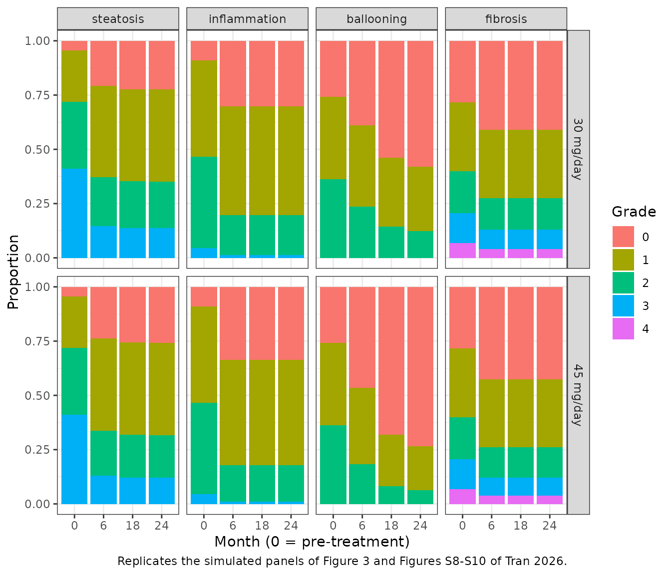
Grade proportions against time with the trial data (Figure 2, Figures S3 to S5)
Replicates the layout of the visual predictive checks: the predicted proportion of each grade over time for placebo and for 30 and 45 mg/day, with the observed proportions from Table S4 as points. The curves are arm-level averages, not a prediction interval.
tc <- arm_course_long(doses = c(0, 30, 45), times = c(0, 0.25, 0.5, 1, 2, 3, 4.5, 6, 9, 12, 15, 18, 21, 24)) |>
  mutate(grade = paste("grade", grade))

obs_points <- comparison_long |>
  left_join(distinct(observed, endpoint, study, arm, dose), by = c("endpoint", "study", "arm")) |>
  mutate(grade = paste("grade", grade))

ggplot(tc, aes(time, prob, colour = factor(dose))) +
  geom_line() +
  geom_point(data = obs_points, aes(y = obs_prob), shape = 1) +
  facet_grid(factor(endpoint, levels = endpoints) ~ grade) +
  labs(
    x = "Month", y = "Proportion", colour = "Dose (mg/day)",
    caption = "Layout of Figure 2 and Figures S3-S5 of Tran 2026; points are Table S4 counts."
  ) +
  theme_bw()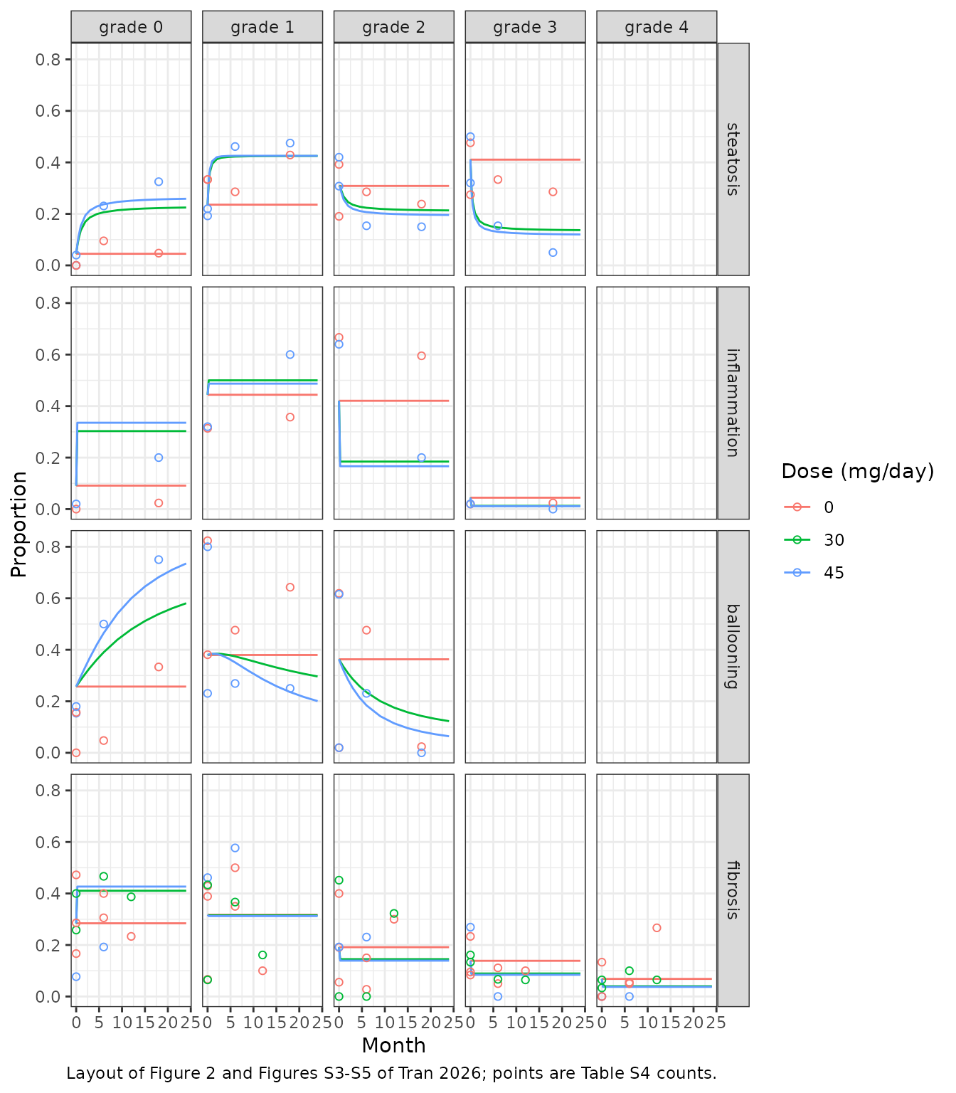
Liver enzymes: Weibull models
Typical trajectories (Figure S2, Figures S6 and S7)
The Weibull models describe arm-mean ALT and AST. At time 0 the
prediction is rmin + wamp (73.0 U/L for ALT, 45.7 U/L for
AST); it then declines towards the plateau rmin (33.9 and
29.6 U/L), quickly on pioglitazone and slowly on placebo.
enz_grid <- expand.grid(time = seq(0, 36, by = 0.25), DOSE_PIO_MGD = c(0, 30))
enz_grid$id <- rep(1:2, each = length(unique(enz_grid$time)))
enz_grid <- enz_grid[order(enz_grid$id, enz_grid$time), ]
enz_grid$evid <- 0

alt_typ <- as.data.frame(solve_quiet(rxode2::zeroRe(alt_ui), enz_grid))
ast_typ <- as.data.frame(solve_quiet(rxode2::zeroRe(ast_ui), enz_grid))
enz_typ <- bind_rows(
  alt_typ |> transmute(time, DOSE_PIO_MGD, enzyme = "ALT", value = alt),
  ast_typ |> transmute(time, DOSE_PIO_MGD, enzyme = "AST", value = ast)
) |>
  mutate(arm = ifelse(DOSE_PIO_MGD > 0, "Pioglitazone", "Placebo"))

ggplot(enz_typ, aes(time, value, colour = arm)) +
  geom_line() +
  facet_wrap(~enzyme, scales = "free_y") +
  labs(
    x = "Month", y = "Arm-mean activity (U/L)", colour = NULL,
    caption = "Typical-value trajectories; compare with the central tendency of Figures S2, S6 and S7 of Tran 2026."
  ) +
  theme_bw()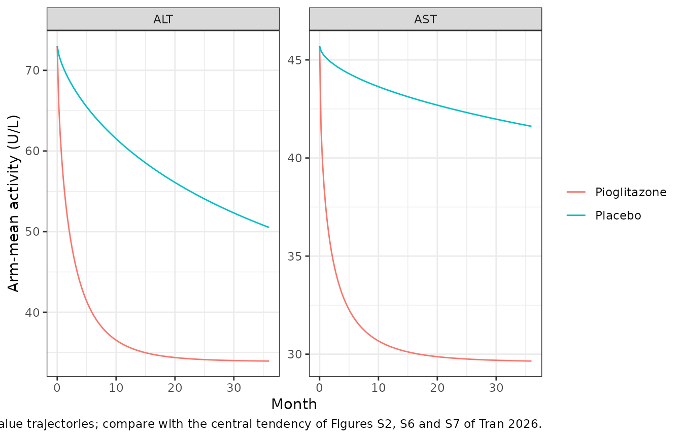
weibull <- function(rmin, wamp, wlambda, wgamma, t) rmin + wamp * exp(-wlambda * t^wgamma)
alt_ref <- ifelse(
  enz_grid$DOSE_PIO_MGD > 0,
  weibull(33.9, 39.1, 0.534, 0.703, enz_grid$time),
  weibull(33.9, 39.1, 0.0689, 0.703, enz_grid$time)
)
ast_ref <- ifelse(
  enz_grid$DOSE_PIO_MGD > 0,
  weibull(29.6, 16.1, 0.694, 0.591, enz_grid$time),
  weibull(29.6, 16.1, 0.0352, 0.591, enz_grid$time)
)

anchors <- enz_typ |>
  filter(time %in% c(0, 6, 12, 24, 36)) |>
  select(enzyme, arm, time, value) |>
  pivot_wider(names_from = time, values_from = value, names_prefix = "month ")
knitr::kable(anchors, digits = 1, caption = "Typical arm-mean ALT and AST (U/L).")| enzyme | arm | month 0 | month 6 | month 12 | month 24 | month 36 |
|---|---|---|---|---|---|---|
| ALT | Placebo | 73.0 | 64.6 | 60.2 | 54.4 | 50.5 |
| ALT | Pioglitazone | 73.0 | 39.9 | 35.7 | 34.2 | 34.0 |
| AST | Placebo | 45.7 | 44.1 | 43.4 | 42.4 | 41.6 |
| AST | Pioglitazone | 45.7 | 31.8 | 30.4 | 29.8 | 29.7 |
stopifnot(
  # The model equals the printed Weibull equation with the Table 2 values.
  all(abs(alt_typ$alt - alt_ref) < 1e-8),
  all(abs(ast_typ$ast - ast_ref) < 1e-8),
  # Pre-treatment value is Baseline + A, whatever the arm.
  all(abs(alt_typ$alt[alt_typ$time == 0] - (33.9 + 39.1)) < 1e-8),
  all(abs(ast_typ$ast[ast_typ$time == 0] - (29.6 + 16.1)) < 1e-8),
  # Placebo declines only modestly (Discussion): ALT still above 50 U/L at
  # 24 months, while pioglitazone brings it to within 1 U/L of the plateau.
  alt_typ$alt[alt_typ$DOSE_PIO_MGD == 0 & alt_typ$time == 24] > 50,
  alt_typ$alt[alt_typ$DOSE_PIO_MGD > 0 & alt_typ$time == 24] - 33.9 < 1,
  ast_typ$ast[ast_typ$DOSE_PIO_MGD > 0 & ast_typ$time == 24] - 29.6 < 1
)
Between-study variability of the arm means (Figures S6 and S7)
A simulated set of 200 placebo and 200 pioglitazone study arms, each
with its own between-study random effects. The residual error in the
models is the per-patient value; the source divides it by
sqrt(N) for an arm of N patients, so it is
added here for arms of 30 patients, the typical arm size of the included
trials (Table S2).
rxode2::rxSetSeed(2026)
n_arms <- 200
arm_n <- 30
vpc_times <- c(0, 1, 2, 3, 6, 9, 12, 18, 24)
vpc_events <- expand.grid(time = vpc_times, id = seq_len(2 * n_arms))
vpc_events$DOSE_PIO_MGD <- ifelse(vpc_events$id > n_arms, 30, 0)
vpc_events$evid <- 0

arm_mean_sim <- function(ui, out, propSd, addSd) {
  sim <- as.data.frame(rxode2::rxSolve(ui, vpc_events))
  ipred <- sim[[out]]
  # Residual for an arm mean of arm_n patients (Methods 2.2.2).
  sd_arm <- sqrt((propSd * ipred)^2 + addSd^2) / sqrt(arm_n)
  sim$value <- ipred + rnorm(nrow(sim), 0, sd_arm)
  sim$arm <- ifelse(sim$DOSE_PIO_MGD > 0, "Pioglitazone", "Placebo")
  sim
}
set.seed(2026)
vpc <- bind_rows(
  arm_mean_sim(rxode2::zeroRe(alt_ui, which = "sigma"), "alt", 0.292, 10.5) |> mutate(enzyme = "ALT"),
  arm_mean_sim(rxode2::zeroRe(ast_ui, which = "sigma"), "ast", 0.352, 0) |> mutate(enzyme = "AST")
)

vpc_q <- vpc |>
  group_by(enzyme, arm, time) |>
  summarise(
    p10 = quantile(value, 0.1), p50 = median(value), p90 = quantile(value, 0.9),
    .groups = "drop"
  )

ggplot(vpc_q, aes(time, p50, colour = arm, fill = arm)) +
  geom_ribbon(aes(ymin = p10, ymax = p90), alpha = 0.2, colour = NA) +
  geom_line() +
  facet_wrap(~enzyme, scales = "free_y") +
  labs(
    x = "Month", y = "Arm-mean activity (U/L)", colour = NULL, fill = NULL,
    caption = "Median and 10th-90th percentiles of simulated arm means (30 patients per arm)."
  ) +
  theme_bw()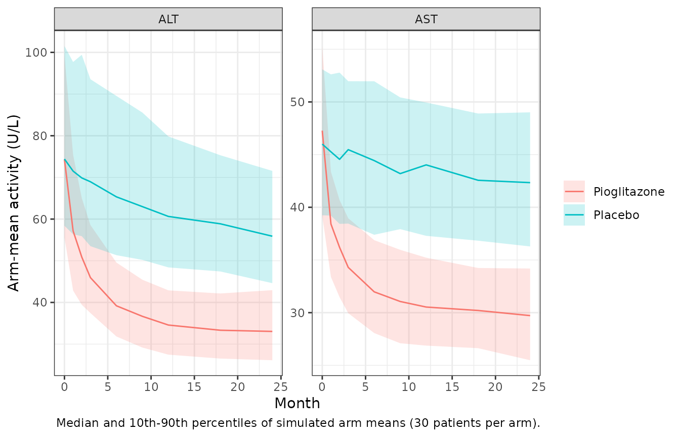
base_spread <- vpc_q |> filter(time == 0)
stopifnot(
  # The median pre-treatment arm sits near the typical Baseline + A. The sum
  # of two log-normal terms has a median about 2% above the sum of their
  # medians, and the median of 400 ALT arms has a standard error of about 2%,
  # so 10% leaves more than 3 standard errors; a wrong amplitude or plateau
  # moves it by tens of percent.
  abs(median(vpc$value[vpc$enzyme == "ALT" & vpc$time == 0]) / 73.0 - 1) < 0.1,
  abs(median(vpc$value[vpc$enzyme == "AST" & vpc$time == 0]) / 45.7 - 1) < 0.1,
  # The 10th-90th percentile band of pre-treatment ALT arm means spans at
  # least 20 U/L, as in the placebo panel of Figure S6.
  diff(unlist(base_spread[base_spread$enzyme == "ALT" & base_spread$arm == "Placebo", c("p10", "p90")])) > 20
)
Assumptions and deviations
-
Threshold indexing. Methods 2.2.1 writes the
cumulative logit as a sum from
beta_0tobeta_m, while the worked steatosis example in the same section starts atbeta_1. The two are the same equation with the indices shifted. Table 1 settles it: it lists one beta per threshold below the top grade (three for steatosis, two for ballooning, four for fibrosis), starting atbeta_0. The no-drug steatosis distribution this gives (0.04, 0.23, 0.31, 0.41) matches the pre-treatment Cusi 2016 pioglitazone arm (0.04, 0.22, 0.42, 0.32).beta_0is stored aslogite0and the increments aslogitstep1,logitstep2, … -
Natural log of the dose. The paper writes
log(dose)without a base. The natural log reproduces the Cusi 2016 45 mg/day arm at 18 months (predicted 0.22, 0.48, 0.20, 0.10 against observed 0.33, 0.48, 0.15, 0.05 for steatosis); base 10 gives 0.09, 0.37, 0.30, 0.24, far from the data. -
ET50, not EC50. Table 1 labels the time constant
“EC50 (month)”, but the equation in the same cell is
Time / (ET50 + Time)and the Discussion calls it ET50. The value is a time in months. -
No drug effect without drug.
log(0)is undefined, so the drug term is set to zero whenDOSE_PIO_MGD = 0. Pre-treatment biopsies must carryDOSE_PIO_MGD = 0: for inflammation and fibrosis, which have no time term, a non-zero dose at time 0 would already apply the full effect. The pre-treatment pioglitazone arms in Table S4 match the no-drug prediction, which supports this coding. - Dose titration. Belfort 2006 and Cusi 2016 gave 30 mg/day for 2 months and 45 mg/day after; Table S4 codes those arms as 45 mg/day, and so do the comparisons here.
-
Random-effect scales. The equation adds
etadirectly to the cumulative logit, soIIV_betais additive on the logit (etalogite0) and is shared by every threshold.IIV_alphais taken as exponential: as an additive SD (0.49 for steatosis against alpha = 0.49) it would make about 16% of patients (24% for inflammation) worse on drug, which contradicts the uniform improvement the paper reports. The Table 2 omegas of the enzyme models are taken as exponential between-study variances; read as additive, the ALT plateau omega would be a 0.5% CV. All OMEGA values are taken as variances. - Random effects of the histology models. They were estimated on resampled virtual patients (500 per arm and time), not on real patients, so they describe the spread of the resampled data rather than real between-patient variability. The models are suited to arm-level grade distributions.
-
Enzyme ‘Baseline’ is the plateau. At
t = 0,exp(0) = 1, so the Table 2 equation gives Baseline + A (73.0 U/L for ALT, 45.7 for AST), which matches the pre-treatment arm means in Figure S2. Astgrows it tends to Baseline (33.9 and 29.6 U/L). The term is therefore stored as the plateaurmin, not as a pre-treatment baseline. - Time units of the enzyme models. Table 2 does not state them. The time axes of Figures 4, 5, S2, S6 and S7 are in months and ET50 of the histology models is in months, so months are used.
- Enzyme drug effect. Pioglitazone changes only the Weibull rate (lambda1 placebo, lambda2 drug). No dose-response was found (Discussion), so any dose above 0 uses lambda2. Methods 2.2.2 says variability was explored on lambda, but Table 2 reports none, so the models carry none.
-
Residual error. Table 2’s proportional and additive
errors are taken as standard deviations (a 29% CV and 10.5 U/L for ALT).
The source divides the residual by
sqrt(N)for an arm ofNpatients; the models store the unweighted SDs, and the simulation above applies the weighting. AST’s additive error was fixed to 0, so the AST model has a proportional term only. -
Ordinal endpoint coding. The histology models use
the rxode2 ordinal endpoint
<score> ~ c(p0, p1, ...). A simulated value ofkis gradek - 1; the grade probabilitiesp0,p1, … are also returned. - Not reproduced. The external validation on 27 Korean MASLD patients at 15 or 30 mg/day (Figures 4 and 5) uses data that are not published.
- No NCA. These are disease-endpoint models with no drug concentration, so there is no PKNCA analysis; the checks above test the equations, the direction and size of the drug effect, and the variability of arm means.