Tacrolimus IR / PR industry meta (Lu 2019)
Source:vignettes/articles/Lu_2019_tacrolimus_industry_meta.Rmd
Lu_2019_tacrolimus_industry_meta.RmdModel and source
- Citation: Lu Z, Bonate P, Keirns J. Population pharmacokinetics of immediate- and prolonged-release tacrolimus formulations in liver, kidney and heart transplant recipients. Br J Clin Pharmacol. 2019;85(8):1692-1703. doi:10.1111/bcp.13952.
- Description: Industry meta-analysis. Two-compartment population PK model for oral tacrolimus immediate-release (IR-T; Prograf, twice daily) and prolonged-release (PR-T; Advagraf / Astagraf XL, once daily) formulations in adult and paediatric liver, kidney, and heart transplant recipients (Lu 2019). Pooled individual-patient data from 8 Astellas Phase II studies (n = 408 patients, 23,176 whole-blood concentration records). Structural model: first-order absorption with formulation-dependent Ka (PR-T ~50% slower than IR-T), fixed absorption lag time, and two-compartment disposition with first-order elimination. Significant covariates: Asian race on CL/F (+59% vs Whites); log-AST on CL/F, Vc/F, Vp/F, and F1 (power normalised at LAST = 3.15, i.e., AST ~= 23.3 IU/L); female sex on Vc/F (-44.6% vs males); albumin on Vc/F and F1; and Asian / Black race on F1 (Asians > Whites > Blacks). Type of organ transplanted and adult-vs-paediatric population had no significant effect on PK parameters.
- Article: https://doi.org/10.1111/bcp.13952
Lu Z, Bonate P, Keirns J. Population pharmacokinetics of immediate- and prolonged-release tacrolimus formulations in liver, kidney and heart transplant recipients. Br J Clin Pharmacol. 2019;85(8):1692-1703. The final-model NONMEM control stream is in the paper’s Supporting Information Appendix A; this vignette uses only the printed equations (Results section 3.2) and the final-model parameter estimates in Table 3.
Population
Lu 2019 pooled individual-patient data from 8 Astellas Phase II studies (Lu 2019 Table 1) of oral tacrolimus in adult and paediatric solid-organ transplant recipients receiving the twice-daily immediate-release formulation (IR-T; Prograf), the once-daily prolonged-release formulation (PR-T; Advagraf in Europe / Astagraf XL in the US), or both formulations across cross-over conversion occasions.
Overall, 23,176 whole-blood tacrolimus concentration records were obtained from 408 patients (Lu 2019 Table 2). Baseline demographics: 276 male / 132 female (32.4 % female); median age 48 years (range 5 - 71; 17 paediatric); median weight 74 kg (range 18.5 - 148.5). Race distribution: White n = 340 (83.3 %), Asian n = 44 (10.8 %), Black n = 24 (5.9 %). The Asian cohort is heterogeneous (Japanese, Chinese, and other Far East groups pooled, including the all-Japanese FJ-506E-KT01 study).
The same information is available programmatically via
rxode2::rxode(readModelDb("Lu_2019_tacrolimus_industry_meta"))$population.
Source trace
The per-parameter origin is recorded as an in-file comment next to
each ini() entry in
inst/modeldb/specificDrugs/Lu_2019_tacrolimus_industry_meta.R.
The table below collects them in one place for review.
| Equation / parameter | Value | Source location |
|---|---|---|
| Two-cmt oral PK, first-order absorption + lag | structural | Lu 2019 Results 3.1 (base model selection); Methods 2.3.2 |
| CL/F typical | 44.3 L/h | Lu 2019 Table 3 ‘CL/F’ |
| Asian race on CL/F | +0.59 | Lu 2019 Table 3 ‘Asian race on CL/F’; Black on CL/F was dropped for lack of precision (Results 3.2) |
| AST on CL/F | -0.318 | Lu 2019 Table 3 ‘AST on CL/F’; equation Results 3.2 ((LAST/3.15)^-0.318) |
| Vc/F typical | 110 L | Lu 2019 Table 3 ‘Vc/F’ |
| Sex on Vc/F | -0.446 | Lu 2019 Table 3 ‘Sex on Vc/F’ (-44.6 % in females) |
| AST on Vc/F | +1.73 | Lu 2019 Table 3 ‘AST on Vc/F’; equation Results 3.2 |
| ALB on Vc/F | +1.03 | Lu 2019 Table 3 ‘ALB on Vc/F’; ALB reference 39 g/L (Methods 2.3.5) |
| Q/F typical | 131 L/h | Lu 2019 Table 3 ‘Q/F’ |
| Vp/F typical | 3180 L | Lu 2019 Table 3 ‘Vp/F’ |
| AST on Vp/F | -0.945 | Lu 2019 Table 3 ‘AST on Vp/F’; equation Results 3.2 |
| Ka typical (IR-T) | 0.375 /h | Lu 2019 Table 3 ‘Ka’ |
| PR-T effect on Ka | 0.499 | Lu 2019 Table 3 ‘Prolonged-release tacrolimus on Ka’ (Ka(PR-T) ~ 50 % of Ka(IR-T)) |
| F1 typical | 1.51 | Lu 2019 Table 3 ‘F1’; relative scaling factor at reference |
| Asian race on F1 | +0.25 | Lu 2019 Table 3 ‘Asian race on F1’ |
| Black race on F1 | -0.433 | Lu 2019 Table 3 ‘Black race on F1’ |
| AST on F1 | +0.74 | Lu 2019 Table 3 ‘AST on F1’ |
| ALB on F1 | +1.04 | Lu 2019 Table 3 ‘ALB on F1’ |
| ALAG1 | 0.44 h | Lu 2019 Table 3 ‘ALAG1’ |
| IPV-CL %CV | 30.9 % | Lu 2019 Table 3 ‘IPV-CL’ |
| IPV-Vc %CV | 106 % | Lu 2019 Table 3 ‘IPV-Vc’ |
| IPV-Q %CV | 39.3 % | Lu 2019 Table 3 ‘IPV-Q’ |
| IPV-Vp %CV | 99 % | Lu 2019 Table 3 ‘IPV-Vp’ |
| IPV-Ka %CV | 35.5 % | Lu 2019 Table 3 ‘IPV-Ka’ |
| IPV-F1 %CV | 30.5 % | Lu 2019 Table 3 ‘IPV-F1’ |
| BOV-F1 %CV | 59.9 % | Lu 2019 Table 3 ‘BOV-F1’ (not encoded; see Assumptions) |
| RV1 (LC-MS/MS) %CV | 21.1 % | Lu 2019 Table 3 ‘RV1’; default in the model file |
| RV2 (immunoassay) %CV | 15.8 % | Lu 2019 Table 3 ‘RV2’; alternative for the FJ-506E-KT01 cohort |
The AST factor is implemented as
exp(theta * (log(AST) - 3.15)), which is mathematically
identical to the paper’s (LAST / 3.15)^theta notation once
the reference centring LAST_ref = 3.15 is taken as the
centring point (not as a dimensionless divisor) - the e-fold rule (“AST
x 2.7 -> exp(theta)”) that the paper’s narrative invokes (Lu 2019
Results 3.2) only holds under this interpretation.
Virtual cohort
The original clinical data are confidential (Astellas internal sources). The cohort below assembles virtual subjects whose covariate distributions approximate Lu 2019 Table 2 baseline demographics and Methods 2.3.5 simulation scenario.
set.seed(20260518)

make_cohort <- function(n, form_label, form_tac_ir,
                        race_label, race_asian, race_black,
                        id_offset = 0L) {
  tibble::tibble(
    id          = id_offset + seq_len(n),
    cohort      = paste(form_label, race_label, sep = " / "),
    FORM_TAC_IR = form_tac_ir,
    RACE_ASIAN  = race_asian,
    RACE_BLACK  = race_black,
    SEXF        = 0L,
    ALB         = 39,
    AST         = 25
  )
}

n_per <- 100L

cohorts <- list(
  make_cohort(n_per, "IR-T", 1L, "White", 0L, 0L, id_offset =   0L),
  make_cohort(n_per, "IR-T", 1L, "Asian", 1L, 0L, id_offset = 100L),
  make_cohort(n_per, "IR-T", 1L, "Black", 0L, 1L, id_offset = 200L),
  make_cohort(n_per, "PR-T", 0L, "White", 0L, 0L, id_offset = 300L),
  make_cohort(n_per, "PR-T", 0L, "Asian", 1L, 0L, id_offset = 400L),
  make_cohort(n_per, "PR-T", 0L, "Black", 0L, 1L, id_offset = 500L)
)

subjects <- dplyr::bind_rows(cohorts)
stopifnot(!anyDuplicated(subjects$id))

# Dosing per Lu 2019 Methods 2.3.5 simulation: IR-T 5 mg BID; PR-T 10 mg QD,
# both at steady state. Simulate the last 24 h of a 14-day regimen.
make_doses <- function(sub_row) {
  is_ir <- sub_row$FORM_TAC_IR == 1L
  if (is_ir) {
    dose_times <- seq(0, 13 * 24, by = 12)
    amt        <- 5
  } else {
    dose_times <- seq(0, 13 * 24, by = 24)
    amt        <- 10
  }
  tibble::tibble(
    id          = sub_row$id,
    time        = dose_times,
    amt         = amt,
    evid        = 1L,
    cmt         = "depot",
    cohort      = sub_row$cohort,
    FORM_TAC_IR = sub_row$FORM_TAC_IR,
    RACE_ASIAN  = sub_row$RACE_ASIAN,
    RACE_BLACK  = sub_row$RACE_BLACK,
    SEXF        = sub_row$SEXF,
    ALB         = sub_row$ALB,
    AST         = sub_row$AST
  )
}

obs_grid <- function(sub_row) {
  is_ir <- sub_row$FORM_TAC_IR == 1L
  obs_t <- if (is_ir) {
    seq(13 * 24, 14 * 24, by = 0.5)
  } else {
    seq(13 * 24, 14 * 24, by = 0.5)
  }
  tibble::tibble(
    id          = sub_row$id,
    time        = obs_t,
    amt         = 0,
    evid        = 0L,
    cmt         = "Cc",
    cohort      = sub_row$cohort,
    FORM_TAC_IR = sub_row$FORM_TAC_IR,
    RACE_ASIAN  = sub_row$RACE_ASIAN,
    RACE_BLACK  = sub_row$RACE_BLACK,
    SEXF        = sub_row$SEXF,
    ALB         = sub_row$ALB,
    AST         = sub_row$AST
  )
}

events <- dplyr::bind_rows(
  lapply(split(subjects, subjects$id), function(s) {
    dplyr::bind_rows(make_doses(s), obs_grid(s))
  })
) |>
  dplyr::arrange(id, time, dplyr::desc(evid))
Simulation
mod <- readModelDb("Lu_2019_tacrolimus_industry_meta")
sim <- rxode2::rxSolve(
  mod,
  events = events,
  keep   = c("cohort", "FORM_TAC_IR", "RACE_ASIAN", "RACE_BLACK")
) |>
  as.data.frame()
#> ℹ parameter labels from comments will be replaced by 'label()'
For deterministic typical-value replications, zero out the random effects:
Replicate published figures
Lu 2019 Figure 3A stratifies simulated trough concentrations by race, formulation, and sex. The chunk below reproduces the race-by-formulation box plot for males at reference AST (25 IU/L) and ALB (39 g/L). Lu 2019 overlays the therapeutic window 5 - 20 ng/mL; the same shaded band is reproduced here.
# Replicates Figure 3A of Lu 2019: simulated trough concentrations by
# race and formulation (male, reference AST = 25 IU/L, ALB = 39 g/L).
trough <- sim |>
  dplyr::group_by(id, cohort) |>
  dplyr::slice_tail(n = 1) |>
  dplyr::ungroup() |>
  tidyr::separate(cohort, into = c("formulation", "race"),
                  sep = " / ", remove = FALSE)

ggplot(trough, aes(x = race, y = Cc, fill = formulation)) +
  annotate("rect", xmin = -Inf, xmax = Inf, ymin = 5, ymax = 20,
           fill = "grey80", alpha = 0.4) +
  geom_boxplot(outlier.shape = NA, position = position_dodge(0.7), width = 0.6) +
  labs(x = "Race", y = "Simulated tacrolimus trough (ng/mL)",
       fill = "Formulation",
       title = "Lu 2019 Figure 3A replication",
       caption = paste(
         "Race x formulation, male, reference AST 25 IU/L and ALB 39 g/L.",
         "Therapeutic window 5 - 20 ng/mL shaded.")) +
  coord_cartesian(ylim = c(0, 35))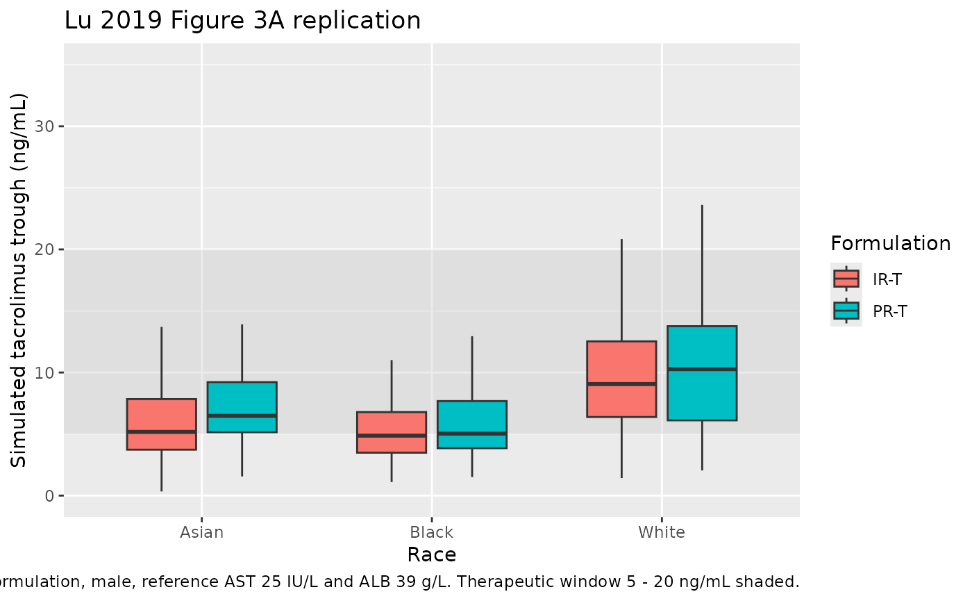
PKNCA validation
Single-dose AUC and Cmax / Tmax / half-life can be derived for the IR-T and PR-T arms separately. For comparability with Lu 2019 Methods 2.3.5 (steady-state simulation), the PKNCA call below uses the final 24-h inter-dose window of the 14-day regimen and reports per-formulation summaries.
sim_nca <- sim |>
  dplyr::filter(!is.na(Cc), time >= 13 * 24) |>
  dplyr::mutate(tau_time = time - 13 * 24) |>
  dplyr::select(id, tau_time, Cc, cohort)

conc_obj <- PKNCA::PKNCAconc(sim_nca, Cc ~ tau_time | cohort + id)

dose_df <- events |>
  dplyr::filter(evid == 1L, time >= 13 * 24, time < 14 * 24) |>
  dplyr::mutate(tau_time = time - 13 * 24) |>
  dplyr::select(id, tau_time, amt, cohort)

dose_obj <- PKNCA::PKNCAdose(dose_df, amt ~ tau_time | cohort + id)

intervals <- data.frame(
  start          = 0,
  end            = 24,
  cmax           = TRUE,
  tmax           = TRUE,
  auclast        = TRUE,
  half.life      = TRUE
)

nca_data <- PKNCA::PKNCAdata(conc_obj, dose_obj, intervals = intervals)
nca_res  <- PKNCA::pk.nca(nca_data)

knitr::kable(
  summary(nca_res),
  caption = "Simulated NCA parameters by race x formulation (last 24 h of steady state)."
)| start | end | cohort | N | auclast | cmax | tmax | half.life |
|---|---|---|---|---|---|---|---|
| 0 | 24 | IR-T / Asian | 100 | 209 [48.1] | 18.3 [43.6] | 1.50 [1.00, 4.50] | 58.9 [49.8] |
| 0 | 24 | IR-T / Black | 100 | 157 [53.1] | 11.9 [45.3] | 1.50 [1.00, 4.50] | 95.0 [79.7] |
| 0 | 24 | IR-T / White | 100 | 279 [45.8] | 20.0 [43.8] | 1.50 [1.00, 4.50] | 81.0 [65.3] |
| 0 | 24 | PR-T / Asian | 100 | 263 [41.1] | 20.0 [44.2] | 2.00 [1.00, 6.00] | 39.7 [24.7] |
| 0 | 24 | PR-T / Black | 100 | 186 [47.9] | 11.8 [44.2] | 2.00 [1.00, 6.50] | 47.0 [30.0] |
| 0 | 24 | PR-T / White | 100 | 323 [42.1] | 21.2 [40.0] | 2.50 [1.00, 6.00] | 52.0 [32.5] |
Comparison against published NCA
Lu 2019 reports the qualitative finding that trough concentrations were within the 5 - 20 ng/mL therapeutic window for typical subjects across race and formulation, with PR-T:IR-T relative bioavailability geometric mean ratio = 95 % (90 % CI 89 - 101 %) on posthoc empirical-Bayes analysis (Results 3.2). Quantitative per-arm NCA tables are not provided in the paper, so the table above is the qualitative match: simulated trough values cluster within the therapeutic window for the reference subject and stratify by race in the published direction (Asians > Whites > Blacks).
Assumptions and deviations
-
Formulation effect on F1 omitted. Lu 2019 prints a
structural F1 equation that includes a formulation term
(1 - (1 - theta_form) * FORMULATION)(Results 3.2). The final-model parameter table (Lu 2019 Table 3) does not list a correspondingProlonged-release tacrolimus on F1row; the abstract characterises the PR-T : IR-T relative- bioavailability geometric-mean ratio (95 %, 90 % CI 89 - 101 %; the 90 % CI crosses 1.0) as a posthoc empirical-Bayes summary, not a structural fixed effect. The model file omits the formulation effect on F1 and keeps the equation formF1 = exp(lfdepot + etalfdepot) * race_f * alb_f * ast_f. -
BOV-F1 (59.9 % CV) not encoded. Lu 2019 reports
between-occasion variability on F1 in Table 3, but the canonical
nlmixr2lib model files carry one subject-level eta per parameter and the
paper does not define an explicit “occasion” indicator. Downstream users
who want to simulate BOV-F1 can add an OCC column and a per-occasion eta
on
lfdepotin their rxode2 event table. -
Residual error: log-additive (LTBS) maps to
lnorm(expSd). Lu 2019 fitted the final model on log-transformed concentrations with an additive residual term (“residual additive error model with the log-transformed tacrolimus concentration data was found to best describe the data”, Results 3.1). The packaged model usesCc ~ lnorm(expSd)withexpSd = 0.211(LC-MS/MS, RV1). For the Japanese cohort study FJ-506E-KT01 (immunoassay, RV2 = 15.8 %), setexpSd = 0.158in the user code or refit with the alternative value. -
AST normalisation
(LAST / 3.15)^thetainterpretation. Lu 2019 Results 3.2 writes the AST factor as(LAST / 3.15)^thetawithLAST = log(AST), “normalized at 3.15 IU/L”. Taken literally as a power oflog(AST) / 3.15the formula does not reproduce the paper’s stated factor magnitudes (e.g., a 2.7-fold AST increase yieldingexp(-0.318) ~= 0.73on CL/F). The mathematically equivalentexp(theta * (LAST - 3.15))form does, so the model uses that form with referenceAST_ref = exp(3.15) ~= 23.3 IU/L. This is a notational interpretation, not a parameter change. - Black race on CL/F not in the final model. Lu 2019 Results 3.2: “Due to the lack of precision of the effect of Black race on tacrolimus CL/F, this parameter was not included in the final model.” The packaged CL/F equation accordingly carries only the Asian race effect (+59 %); Black race on CL/F is left at 0.
- Bootstrap convergence. Lu 2019 reports 491 of 1000 bootstrap runs with minimization terminated (skipped), 8 with estimates near a boundary. The remaining 501 successful runs gave parameter medians and 95 % CIs in close agreement with the point estimates; the packaged model uses the original point estimates, not the bootstrap medians.
- Type of organ transplanted and adult-vs-paediatric population not included. Lu 2019 Results 3.2: type of organ transplanted (kidney vs liver vs heart) had no significant effect on principal PK parameters and adult-vs-paediatric population effects were underpowered (4.2 % paediatric). Both factors were therefore excluded from the final model and the packaged model.
- CYP3A4 / CYP3A5 / P-gp genotype not modelled. Lu 2019 Discussion notes higher CYP3A5 polymorphism in African-Americans as a likely mechanism for the racial bioavailability differences, but CYP3A4 / CYP3A5 / P-gp variants were not collected as covariates in the study databases and so are not in the final model or the packaged model. Downstream users who want a genotype-stratified PK should consult Storset 2014 or other CYP3A5-genotyped tacrolimus models in nlmixr2lib.