Hydrocortisone and 17-OHP in dried blood spots (Stachanow 2023)
Source:vignettes/articles/Stachanow_2023_hydrocortisone.Rmd
Stachanow_2023_hydrocortisone.RmdModel and source
- Citation: Stachanow V, Neumann U, Blankenstein O, Alder-Baerens N, Bindellini D, Hindmarsh P, Ross RJ, Whitaker MJ, Melin J, Huisinga W, Michelet R, Kloft C. Model-Informed Target Morning 17alpha-Hydroxyprogesterone Concentrations in Dried Blood Spots for Pediatric Congenital Adrenal Hyperplasia Patients. Pharmaceuticals (Basel). 2023;16(3):464. doi:10.3390/ph16030464. Cortisol PK layer from Stachanow V, Neumann U, Blankenstein O, Bindellini D, Melin J, Ross R, Whitaker MJ, Huisinga W, Michelet R, Kloft C. Exploring Dried Blood Spot Cortisol Concentrations as an Alternative for Monitoring Pediatric Adrenal Insufficiency Patients: A Model-Based Analysis. Front Pharmacol. 2022;13:819590. doi:10.3389/fphar.2022.819590.
- Description: Pediatric PK/PD model of oral hydrocortisone (Alkindi granules) in young children and infants with congenital adrenal hyperplasia: total plasma cortisol from a two-compartment model with saturable (Michaelis-Menten) absorption, saturable corticosteroid-binding-globulin and linear albumin plasma binding acting on unbound cortisol, and allometric weight scaling (Stachanow 2022) inhibits the synthesis of 17-alpha-hydroxyprogesterone (17-OHP) measured in venous dried blood spots through an indirect-response model whose baseline is the subject’s observed pre-dose DBS 17-OHP (Stachanow 2023).
- Article: https://doi.org/10.3390/ph16030464 (open access; the supplement holds the PK/PD equations and the NONMEM code)
- Cortisol PK source: https://doi.org/10.3389/fphar.2022.819590 (open access; Table 1 and the supplementary NONMEM code)
Stachanow 2023 links total plasma cortisol after a morning dose of hydrocortisone granules (Alkindi) to 17-alpha-hydroxyprogesterone (17-OHP) measured in venous dried blood spots (DBS) in young children and infants with congenital adrenal hyperplasia (CAH). Cortisol inhibits the zero-order synthesis of 17-OHP (indirect-response model, Imax = 1, Hill = 1). The PD was fitted sequentially on top of the authors’ earlier pediatric cortisol PK model (Stachanow 2022): each child’s individual PK parameters were data items. The packaged model therefore carries the 2022 typical values and between-subject variability for the cortisol layer, so that it can simulate new children:
- two-compartment disposition of unbound cortisol;
- saturable (Michaelis-Menten) absorption from the depot;
- saturable binding to corticosteroid-binding globulin (CBG) and linear binding to albumin;
- allometric weight scaling to 70 kg.
The paper used the model to derive a target range for morning DBS 17-OHP. It simulated physiological 17-OHP from healthy children’s 24-hour cortisol profiles and multiplied the 6-8 a.m. values by 3 and by 5. That calculation is reproduced at the end of this article.
Dosing is in nmol of hydrocortisone and concentrations are in nmol/L, the units in which the source models were fitted. To convert a dose in mg, use the molar mass of hydrocortisone, 362.46 g/mol (1 mg = 2759 nmol). The molar mass is not stated in the papers.
Population
The PK/PD model was fitted to 18 children from the phase 3 Alkindi trial (NCT02720952; Charite Berlin): 12 young children aged 2-6 years and 6 infants aged 28 days-2 years. They had a median age of 2.5 years (4 months-5 years) and a median weight of 15 kg (7-21 kg) (Stachanow 2023 Table S1). The trial enrolled 23 CAH patients and 1 patient with hypopituitarism. Each child received one individualised morning dose of 1-4 mg (Stachanow 2022 Methods). Plasma cortisol was sampled before the dose and at 1 h and 4 h, with two further samples in the young children. The PD dataset had 88 venous DBS 17-OHP concentrations, 22 of them below the LLOQ of 1.3 nmol/L; these were handled with the M3 method. Sex and race were not reported.
The cortisol PK model (Stachanow 2022) pooled 30 dexamethasone-suppressed healthy adults with 24 pediatric patients, including 6 neonates who are not part of the PD cohort.
str(readModelDb("Stachanow_2023_hydrocortisone")()$population)
#> List of 12
#>  $ species       : chr "human"
#>  $ n_subjects    : int 18
#>  $ n_studies     : int 1
#>  $ age_range     : chr "4 months - 5 years (cohorts: young children 2-6 years, infants 28 days - 2 years)"
#>  $ age_median    : chr "2.5 years"
#>  $ weight_range  : chr "7-21 kg"
#>  $ weight_median : chr "15 kg"
#>  $ disease_state : chr "Pediatric adrenal insufficiency, predominantly congenital adrenal hyperplasia (the phase 3 trial enrolled 23 CA"| __truncated__
#>  $ dose_range    : chr "Single individualised morning oral dose of hydrocortisone granules (Alkindi), 1-4 mg (Stachanow 2022 Methods)."
#>  $ regions       : chr "Germany (Charite Berlin)"
#>  $ n_observations: chr "88 venous DBS 17-OHP concentrations (22 below the LLOQ of 1.3 nmol/L, handled with the M3 method) and 88 plasma"| __truncated__
#>  $ notes         : chr "Stachanow 2023 Section 2.1.1 and Table S1; phase 3 Alkindi trial NCT02720952. Sex and race are not reported. Th"| __truncated__
Source trace
Every ini() value carries an in-file comment pointing at
its source. They are collected here.
| Equation / parameter | Value | Source location |
|---|---|---|
lcl (CL, 70 kg) |
400 L/h | Stachanow 2022 Table 1 |
lvc (Vc, 70 kg) |
10.6 L | Stachanow 2022 Table 1 |
lq (Q, 70 kg) |
160 L/h | Stachanow 2022 Table 1 |
lvp (Vp, 70 kg) |
124 L | Stachanow 2022 Table 1 |
ltmax_abs (Vmax) |
21388 nmol/h | Stachanow 2022 Table 1 |
lkt_abs (Km) |
4810 nmol (fixed) | Stachanow 2022 Table 1 |
lfdepot (F) |
1 (fixed) | Stachanow 2022 Table 1 |
e_wt_cl_q, e_wt_vc_vp
|
0.75, 1 (fixed) | Stachanow 2022 Methods; supplement $PK
|
lkcbg (Kd for CBG) |
9.71 nmol/L (fixed) | Stachanow 2022 Table 1 |
nsalb (NSAlb) |
4.15 (fixed) | Stachanow 2022 Table 1 |
lbs_cbg (binding sites per CBG) |
1 (fixed) | Stachanow 2022 supplement $THETA 6 |
bmax |
TRANSCORTIN * 1000 / 52 nmol/L |
Stachanow 2022 supplement $PK
(CBGmol = CBG2*1000/52) |
lrbase_cortisol (pre-dose plasma cortisol) |
9.41 nmol/L | Stachanow 2022 Table 1 (BASEchild, pla) |
lkdeg |
1.22 1/h | Stachanow 2023 Table 1 |
lic50 |
21.0 nmol/L | Stachanow 2023 Table 1 |
imax, hill
|
1, 1 (fixed) | Stachanow 2023 Table 1 |
etalcl, etaltmax_abs,
etalkt_abs, etalfdepot
|
0.0644, 0.196, 0.270, 0.123 | Stachanow 2022 Table 1 (25.8, 46.5, 55.7, 36.1 %CV) |
etalbs_cbg |
0.049 (fixed) | Stachanow 2022 supplement $OMEGA 6 |
etalrbase_cortisol |
0.144^2 (fixed) | Stachanow 2022 supplement (ETA(13)*THETA(14), omega
1) |
etalkdeg |
0.0025 (fixed) | Stachanow 2023 supplement $OMEGA; Table 1 5.0 %CV |
etalic50 |
0.733 | Stachanow 2023 Table 1 (104 %CV) |
etalrbase |
0.381^2 (fixed) | Stachanow 2023 supplement (ETA(3)*THETA(3), omega
1) |
expSd (plasma cortisol) |
0.144 | Stachanow 2022 Table 1 (14.4 %) |
expSd_ohp17_dbs |
0.381 | Stachanow 2023 Table 1 (38.1 %) |
d/dt(depot), d/dt(central),
d/dt(peripheral1)
|
n/a | Stachanow 2022 supplement, differential equations; Stachanow 2023
supplement $DES
|
| unbound cortisol (quadratic) | n/a | Stachanow 2022 supplement A_u equation; Stachanow 2023
$DES AUP
|
d/dt(effect), ksyn = rbase * kdeg
|
n/a | Stachanow 2023 supplement $PK / $DES
|
central(0), effect(0)
|
n/a | Stachanow 2023 supplement A_0(2) = IBASE*V1,
A_0(5) = OHPBASE
|
Virtual cohort
The observed data are not public. The virtual cohort below follows Table S1 and Figure 3A of the paper:
- Weight: log-normal around 15 kg, truncated to 7-21 kg.
- CBG: 22.4 mg/L for every child. This is the value the authors used when CBG was not measured; the pediatric CBG distribution is not reported.
- Baseline DBS 17-OHP: log-normal with the cohort median of 14.4 nmol/L (Section 2.3) and a log-scale SD of 1. The SD was chosen by the maintainers so the draws span roughly the 3-160 nmol/L of the Figure 3A baselines.
- Dose: three arms at the trial’s dose range, 1, 2 and 4 mg, given at 0 h (morning), with 150 children per arm.
# set.seed() fixes R's draws of the covariates. rxode2's own random-effect
# draws are seeded per solver thread, so assertions below are written to hold
# for any cohort the model can produce.
set.seed(20231)
mw_hc <- 362.46 # g/mol, hydrocortisone (not stated in the source papers)
obs_times <- c(seq(0, 1, by = 0.125), seq(1.25, 4, by = 0.25), seq(4.5, 10, by = 0.5))

make_cohort <- function(n, dose_mg, id_offset = 0L) {
  subj <- tibble(
    id = id_offset + seq_len(n),
    WT = pmin(pmax(exp(rnorm(n, log(15), 0.3)), 7), 21),
    TRANSCORTIN = 22.4,
    OHP17_DBS_BL = exp(rnorm(n, log(14.4), 1)),
    dose_group = paste(dose_mg, "mg")
  )
  doses <- subj |>
    mutate(time = 0, amt = dose_mg * 1e6 / mw_hc, evid = 1L, cmt = "depot", dvid = NA_integer_)
  obs <- subj |>
    tidyr::crossing(time = obs_times) |>
    mutate(amt = 0, evid = 0L, cmt = "central", dvid = 1L)
  bind_rows(doses, obs) |> arrange(id, time, desc(evid))
}

events <- bind_rows(
  make_cohort(150, 1, id_offset = 0L),
  make_cohort(150, 2, id_offset = 150L),
  make_cohort(150, 4, id_offset = 300L)
)
stopifnot(!anyDuplicated(unique(events[, c("id", "time", "evid")])))
The model has two observed endpoints (Cc and
ohp17_dbs), so the observation rows carry
dvid = 1. Both endpoints come back as columns of every
solved row.
Simulation
mod <- rxode2::rxode2(readModelDb("Stachanow_2023_hydrocortisone"))
#> ℹ parameter labels from comments will be replaced by 'label()'
sim <- rxode2::rxSolve(mod, events = events, keep = c("dose_group", "OHP17_DBS_BL")) |>
  as.data.frame()

mod_typical <- rxode2::zeroRe(mod)
typ_events <- bind_rows(lapply(c(1, 2, 4), function(d) {
  make_cohort(1, d, id_offset = d)
})) |>
  mutate(WT = 15, OHP17_DBS_BL = 14.4)
typ_events <- typ_events |>
  filter(evid == 1) |>
  bind_rows(
    typ_events |>
      filter(evid == 0) |>
      distinct(id, .keep_all = TRUE) |>
      select(-time) |>
      tidyr::crossing(time = seq(0, 12, by = 0.05))
  ) |>
  arrange(id, time, desc(evid))
sim_typ <- rxode2::rxSolve(mod_typical, events = typ_events, keep = "dose_group") |>
  as.data.frame()
#> ℹ omega/sigma items treated as zero: 'etalcl', 'etaltmax_abs', 'etalkt_abs', 'etalfdepot', 'etalbs_cbg', 'etalrbase_cortisol', 'etalkdeg', 'etalic50', 'etalrbase'
#> Warning: multi-subject simulation without without 'omega'
Replicate published figures
Figure 3A: the U-shaped 17-OHP time course
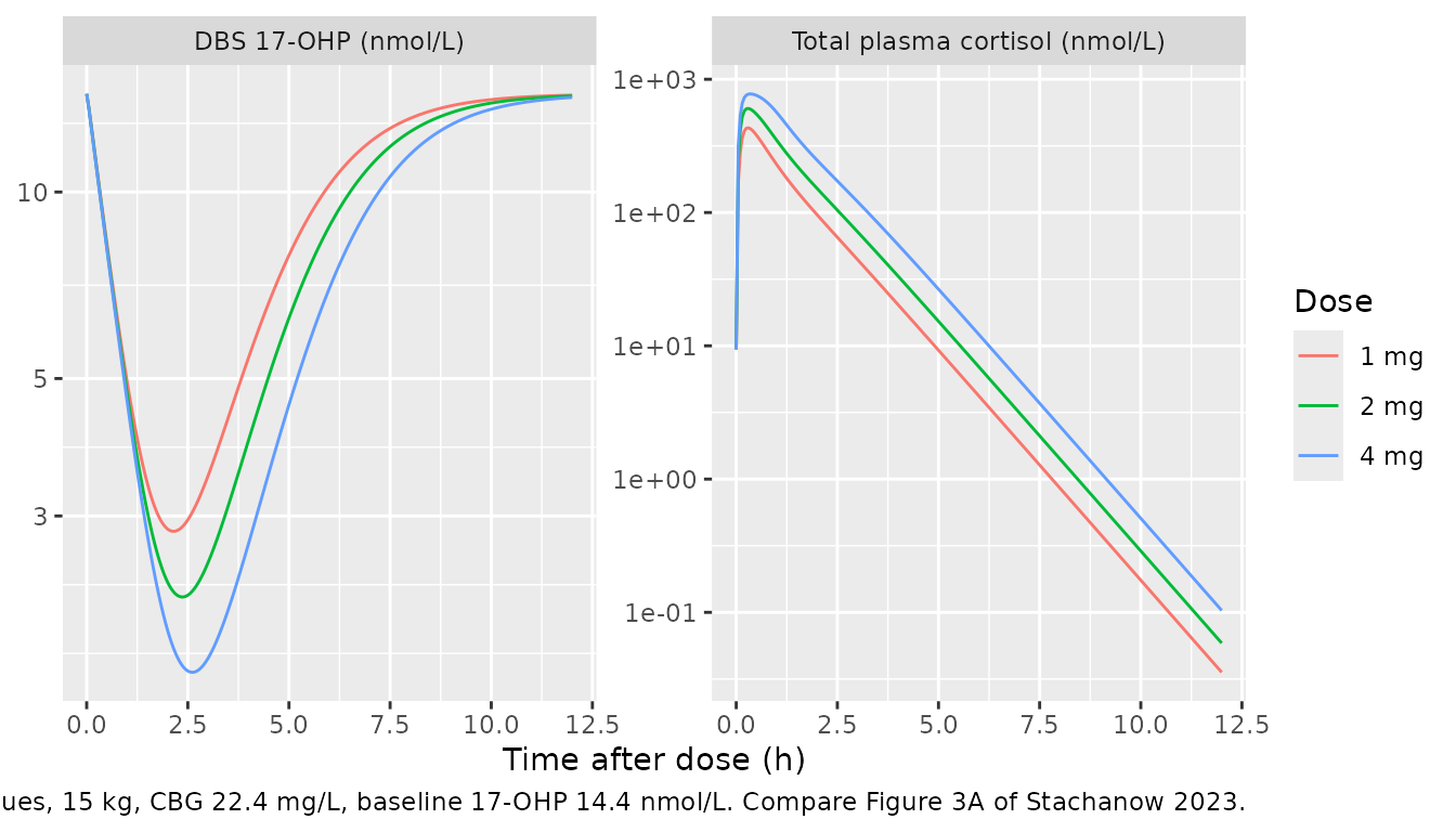
The paper’s Figure 3A shows observed DBS 17-OHP falling after the morning dose and rising again as plasma cortisol declines. Most profiles reach their minimum between about 1 and 4 h and approach baseline by 6-8 h. The typical-value simulation reproduces that shape for a 15-kg child with the median baseline of 14.4 nmol/L.
sim_typ |>
  select(time, dose_group, Cc, ohp17_dbs) |>
  pivot_longer(c(Cc, ohp17_dbs), names_to = "output", values_to = "conc") |>
  mutate(output = recode(output,
    Cc = "Total plasma cortisol (nmol/L)",
    ohp17_dbs = "DBS 17-OHP (nmol/L)"
  )) |>
  ggplot(aes(time, conc, colour = dose_group)) +
  geom_line() +
  facet_wrap(~output, scales = "free_y") +
  scale_y_log10() +
  labs(
    x = "Time after dose (h)", y = NULL, colour = "Dose",
    caption = "Typical values, 15 kg, CBG 22.4 mg/L, baseline 17-OHP 14.4 nmol/L. Compare Figure 3A of Stachanow 2023."
  )
u_shape <- sim_typ |>
  group_by(dose_group) |>
  summarise(
    t_nadir = time[which.min(ohp17_dbs)],
    nadir = min(ohp17_dbs),
    at_8h = ohp17_dbs[which.min(abs(time - 8))],
    .groups = "drop"
  )
knitr::kable(u_shape |> rename(
  "Dose" = dose_group, "Time of nadir (h)" = t_nadir,
  "Nadir 17-OHP (nmol/L)" = nadir, "17-OHP at 8 h (nmol/L)" = at_8h
), digits = 2)| Dose | Time of nadir (h) | Nadir 17-OHP (nmol/L) | 17-OHP at 8 h (nmol/L) |
|---|---|---|---|
| 1 mg | 2.15 | 2.83 | 13.15 |
| 2 mg | 2.35 | 2.22 | 12.52 |
| 4 mg | 2.60 | 1.68 | 11.51 |
stopifnot(
  # The nadir falls inside the 1-4 h window where Figure 3A profiles bottom out.
  all(u_shape$t_nadir > 1 & u_shape$t_nadir < 4),
  # Suppression is substantial (Figure 3A: profiles fall several-fold) ...
  all(u_shape$nadir < 0.5 * 14.4),
  # ... and the profile has recovered most of the way by 8 h.
  all(u_shape$at_8h > 0.5 * 14.4)
)
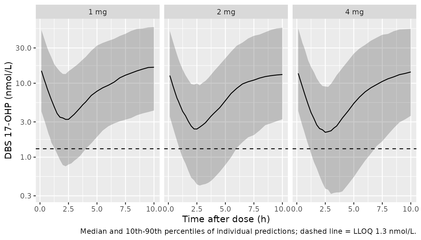
Cohort profiles (compare Figure 3A and Supplementary Figure S3)
sim |>
  filter(time > 0) |>
  group_by(time, dose_group) |>
  summarise(
    Q10 = quantile(ohp17_dbs, 0.10), Q50 = median(ohp17_dbs),
    Q90 = quantile(ohp17_dbs, 0.90), .groups = "drop"
  ) |>
  ggplot(aes(time, Q50)) +
  geom_ribbon(aes(ymin = Q10, ymax = Q90), alpha = 0.25) +
  geom_line() +
  geom_hline(yintercept = 1.3, linetype = "dashed") +
  facet_wrap(~dose_group) +
  scale_y_log10() +
  labs(
    x = "Time after dose (h)", y = "DBS 17-OHP (nmol/L)",
    caption = "Median and 10th-90th percentiles of individual predictions; dashed line = LLOQ 1.3 nmol/L."
  )
PKNCA validation
Neither paper reports NCA of plasma cortisol, so the PKNCA block below documents the simulated exposure by dose group. It has no published comparator. Cortisol is the only output where NCA applies; 17-OHP is endogenous and is checked with the PD tests below. The pre-dose plasma cortisol (the child’s residual cortisol, 9.41 nmol/L typical) decays from time 0 and is included in the AUC, as it is in the model.
sim_nca <- sim |>
  dplyr::filter(!is.na(Cc)) |>
  dplyr::select(id, time, Cc, dose_group)

conc_obj <- PKNCA::PKNCAconc(sim_nca, Cc ~ time | dose_group + id)
dose_df <- events |>
  dplyr::filter(evid == 1) |>
  dplyr::select(id, time, amt, dose_group)
dose_obj <- PKNCA::PKNCAdose(dose_df, amt ~ time | dose_group + id)
intervals <- data.frame(
  start = 0, end = 10, cmax = TRUE, tmax = TRUE, auclast = TRUE
)
nca_res <- PKNCA::pk.nca(PKNCA::PKNCAdata(conc_obj, dose_obj, intervals = intervals))

nca_sum <- as.data.frame(nca_res) |>
  filter(PPTESTCD %in% c("cmax", "tmax", "auclast")) |>
  group_by(dose_group, PPTESTCD) |>
  summarise(median = median(PPORRES), .groups = "drop") |>
  pivot_wider(names_from = PPTESTCD, values_from = median)
nca_sum |>
  rename(
    "Dose" = dose_group, "Cmax (nmol/L)" = cmax,
    "Tmax (h)" = tmax, "AUC0-10 (nmol*h/L)" = auclast
  ) |>
knitr::kable(digits = 2, caption = "Median simulated plasma cortisol NCA by dose group.")| Dose | AUC0-10 (nmol*h/L) | Cmax (nmol/L) | Tmax (h) |
|---|---|---|---|
| 1 mg | 623.87 | 468.44 | 0.25 |
| 2 mg | 926.18 | 596.05 | 0.25 |
| 4 mg | 1415.55 | 759.59 | 0.38 |
# Saturable CBG binding makes total cortisol exposure LESS than dose
# proportional: a doubled dose frees a larger unbound fraction, which is
# cleared faster. A mis-coded binding term (e.g. linear) would give a ratio
# of about 2.
auc_ratio <- nca_sum$auclast[nca_sum$dose_group == "4 mg"] /
  nca_sum$auclast[nca_sum$dose_group == "2 mg"]
stopifnot(auc_ratio > 1.1, auc_ratio < 1.9)
The 4 mg / 2 mg AUC ratio is 1.53, less than dose-proportional, as expected from saturable CBG binding.
PD and binding checks
Binding model
The unbound amount in model() is the positive root of
the quadratic for saturable CBG plus linear albumin binding. At any
total concentration it must satisfy
C_total = C_u (1 + NSAlb) + Bmax C_u / (Kd + C_u).
At trace concentrations the CBG-bound share of plasma cortisol tends to (Bmax/Kd) / (1 + NSAlb + Bmax/Kd) = 89.6 % at 22.4 mg/L CBG. Stachanow 2022 reports CBG binding of “approximately 90%” at the LLOQ, in its whole-blood fractions.
th <- mod$theta
kd <- exp(th[["lkcbg"]])
ns <- th[["nsalb"]]
bmax <- 22.4 * 1000 / 52
chk_bind <- sim_typ |>
  filter(dose_group == "4 mg", time > 0) |>
  mutate(
    vc = 10.6 * 15 / 70,
    cu = central_u / vc,
    resid = (cu * (1 + ns) + bmax * cu / (kd + cu)) / Cc - 1
  )
stopifnot(max(abs(chk_bind$resid)) < 1e-6)

frac_cbg_trace <- (bmax / kd) / (1 + ns + bmax / kd)
frac_cbg_peak <- with(
  chk_bind[which.max(chk_bind$Cc), ],
  bmax * cu / (kd + cu) / Cc
)
stopifnot(abs(frac_cbg_trace - 0.90) < 0.01)
At the 4-mg peak (776 nmol/L total) the CBG-bound fraction falls to 49 %, compared with 89.6 % at trace concentrations. Stachanow 2022 describes the same saturation.
Steady state without cortisol
With no cortisol, inh = 1 and 17-OHP must stay at its
baseline, because ksyn = baseline * kdeg.
ev_ss <- data.frame(
  id = 1, time = seq(0, 24, by = 1), amt = 0, evid = 0L, cmt = "central", dvid = 1L,
  WT = 15, TRANSCORTIN = 22.4, OHP17_DBS_BL = 14.4
)
ss <- rxode2::rxSolve(mod_typical, events = ev_ss, params = c(lrbase_cortisol = log(1e-8))) |>
  as.data.frame()
#> ℹ omega/sigma items treated as zero: 'etalcl', 'etaltmax_abs', 'etalkt_abs', 'etalfdepot', 'etalbs_cbg', 'etalrbase_cortisol', 'etalkdeg', 'etalic50', 'etalrbase'
stopifnot(max(abs(ss$ohp17_dbs / 14.4 - 1)) < 1e-4)
Figure 6: derived morning DBS 17-OHP target range
For Step C the authors drove the PD with plasma cortisol from 28 healthy children aged 5-9 years, sampled every 20 minutes over 24 h (Figure 2). They started the 17-OHP compartment at the median baseline of 14.4 nmol/L, ran 1000 simulations, and took the physiological DBS 17-OHP at 6-8 a.m. Those values were multiplied by 3 and by 5 to approximate the target range. The interquartile range of the pooled values was 2.1-8.3 nmol/L, median 4.4 nmol/L.
The individual profiles are not published. The maintainers digitised
the median profile (the blue line in Figure 2) at the
72 sampling times. Below, the packaged model’s PD layer is driven by
that profile, with between-subject variability on IC50 and kdeg. The PD
layer is written out as an rxode2 model whose input CORT is
the cortisol concentration. Its parameters are read from the packaged
model, and a first check confirms it reproduces the packaged model’s
17-OHP when fed the packaged model’s own cortisol.
pd_only <- rxode2::rxode2({
  kdeg <- exp(lkdeg + etalkdeg)
  ic50 <- exp(lic50 + etalic50)
  rbase <- OHP17_DBS_BL * exp(etalrbase)
  ksyn <- rbase * kdeg
  inh <- 1 - imax * CORT^hill / (ic50^hill + CORT^hill)
  d/dt(effect) <- ksyn * inh - kdeg * effect
  effect(0) <- rbase
  ohp17_dbs <- effect
})
pd_par <- c(
  lkdeg = th[["lkdeg"]], lic50 = th[["lic50"]],
  imax = th[["imax"]], hill = th[["hill"]],
  etalkdeg = 0, etalic50 = 0, etalrbase = 0
)

# Equivalence: drive pd_only with the packaged model's own typical cortisol
# (2 mg, dense 0.05-h grid, linear interpolation) and compare 17-OHP.
drv <- sim_typ |> filter(dose_group == "2 mg")
pd_chk <- rxode2::rxSolve(
  pd_only,
  params = pd_par,
  events = data.frame(id = 1, time = drv$time, evid = 0L, CORT = drv$Cc, OHP17_DBS_BL = 14.4),
  covsInterpolation = "linear"
) |> as.data.frame()
rel_diff <- pd_chk$ohp17_dbs / drv$ohp17_dbs - 1
stopifnot(max(abs(rel_diff)) < 0.02)
The PD-only layer matches the packaged model within 0.046 %, the error from interpolating cortisol linearly on the 0.05-h grid.
# Median plasma cortisol of 28 healthy children aged 5-9 years, digitised by
# the maintainers from Figure 2 of Stachanow 2023 at the 20-minute sampling
# grid (00:00 to 23:40), nmol/L.
cort_median <- c(
  88, 153, 173, 178, 207, 212, 248, 249, 226, 217, 240, 294, 341, 345, 425, 427,
  399, 454, 455, 388, 423, 449, 500, 444, 471, 504, 408, 356, 349, 312, 310, 291,
  287, 285, 318, 288, 306, 328, 368, 362, 337, 291, 258, 227, 252, 281, 272, 260,
  224, 220, 224, 270, 220, 225, 241, 226, 187, 194, 174, 161, 131, 116, 113, 113,
  104, 92, 77, 80, 71, 70, 94, 95
)
clock <- seq(0, by = 1 / 3, length.out = length(cort_median))

n_sim <- 200
om <- mod$omega
eta_draw <- data.frame(
  id = seq_len(n_sim),
  etalic50 = rnorm(n_sim, 0, sqrt(om["etalic50", "etalic50"])),
  etalkdeg = rnorm(n_sim, 0, sqrt(om["etalkdeg", "etalkdeg"]))
)
pd_ev <- tidyr::crossing(id = seq_len(n_sim), data.frame(time = clock, CORT = cort_median)) |>
  mutate(evid = 0L, OHP17_DBS_BL = 14.4) |>
  left_join(eta_draw, by = "id")
pd_sim <- rxode2::rxSolve(
  pd_only,
  params = pd_par[c("lkdeg", "lic50", "imax", "hill", "etalrbase")],
  events = pd_ev,
  covsInterpolation = "linear",
  keep = c("CORT")
) |>
  as.data.frame()

morning <- pd_sim |> filter(time >= 6, time <= 8)
target <- c(3 * morning$ohp17_dbs, 5 * morning$ohp17_dbs)
fig6 <- tibble::tibble(
  Statistic = c("25th percentile", "Median", "75th percentile"),
  `Stachanow 2023 (nmol/L)` = c(2.1, 4.4, 8.3),
  `Simulated (nmol/L)` = unname(quantile(target, c(0.25, 0.5, 0.75)))
)
knitr::kable(fig6, digits = 2, caption = "Derived morning (6-8 a.m.) DBS 17-OHP target range: physiological x 3 and x 5, pooled.")| Statistic | Stachanow 2023 (nmol/L) | Simulated (nmol/L) |
|---|---|---|
| 25th percentile | 2.1 | 1.36 |
| Median | 4.4 | 2.47 |
| 75th percentile | 8.3 | 4.69 |
# Quasi-steady state: kdeg = 1.22 1/h makes 17-OHP track cortisol within
# about an hour, so at 6-8 a.m. the solve sits close to the closed form
# baseline * IC50 / (IC50 + C) for each subject.
qss <- morning |>
  select(id, time, CORT, ohp17_dbs) |>
  left_join(eta_draw, by = "id") |>
  mutate(qss = 14.4 * exp(th[["lic50"]] + etalic50) / (exp(th[["lic50"]] + etalic50) + CORT))
stopifnot(abs(median(qss$ohp17_dbs / qss$qss) - 1) < 0.15)
ggplot(data.frame(target = target), aes(x = "", y = target)) +
  geom_boxplot(outlier.shape = NA, coef = 0, fill = "grey85") +
  geom_hline(yintercept = c(1.3, 3.9), colour = "red") +
  coord_cartesian(ylim = c(0, 15)) +
  labs(
    x = "Time: 6-8 a.m.", y = "DBS 17-OHP morning target (nmol/L)",
    caption = "Box: IQR and median of simulated physiological x 3 and x 5.\nRed: expected range 12-36 / 9.29 (Stachanow 2023 Section 3.3)."
  )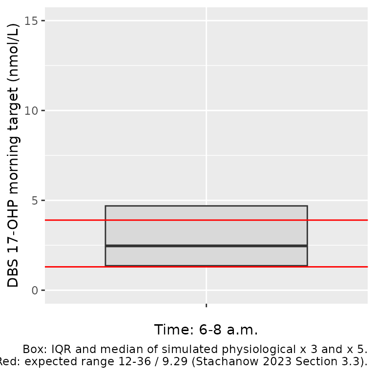
The simulated range is lower than the published one: its median is about 0.56 of the paper’s 4.4 nmol/L. The 17-OHP layer itself reproduces the packaged model exactly (check above), so the gap comes from the cortisol input:
- The paper drove each simulation with one of the 28 individual cortisol profiles; only the median profile can be recovered from Figure 2.
- At quasi-steady state the morning 17-OHP is
14.4 * IC50 / (IC50 + C). With the median morning cortisol of about 450 nmol/L and IC50 = 21 nmol/L, that gives about 0.64 nmol/L, or a target median of about 2.6 nmol/L. The published 4.4 nmol/L would need a typical morning cortisol of about 250 nmol/L, which is below the Figure 2 median between 6 and 8 a.m.
The paper does not state how the cortisol input was aligned in time or whether the 17-OHP baseline carried its variability in Step C. The maintainers have not been able to close the gap from the published information, and the parameters have not been adjusted to match. The simulated range still lies in the same order of magnitude as the paper’s calculated “expected” range of 1.3-3.9 nmol/L (red lines), which was the paper’s plausibility criterion.
Assumptions and deviations
- Cortisol PK carried from Stachanow 2022. The 2023 fit used each child’s individual PK estimates from the 2022 model as data. The packaged model carries the 2022 typical values and variability (Table 1, sampling importance resampling medians), so it simulates new children rather than the fitted 18.
-
Cortisol association with red blood cells is
omitted. The 2022 model’s RBC compartment and blood-volume term
(
Vdelta) produce DBS cortisol. The 2023 PD reads total plasma cortisol only, so that compartment does not affect any output here. DBS cortisol belongs to an extraction of Stachanow 2022 itself. -
CBG is a covariate (
TRANSCORTIN, mg/L). Measured CBG was used for the pediatric data; when CBG was not measured the authors used 22.4 mg/L, which this article uses throughout. - Pre-dose plasma cortisol is a typical value. The 2022 model used each child’s observed pre-dose cortisol (or 9.41 nmol/L when unobserved), with a log-normal deviation whose SD equals the residual SD. The packaged model uses 9.41 nmol/L with that deviation. The baseline is residual cortisol that decays from time 0 (CAH patients make little cortisol), not a steady state. The peripheral compartment starts empty, as in the source code.
-
17-OHP baseline is a covariate,
OHP17_DBS_BL. As in the source, the baseline is the child’s observed pre-dose DBS 17-OHP, with a log-normal deviation whose SD equals the residual SD (OHPBASE = BASEDV*EXP(ETA(3)*THETA(3)), omega 1). Table 1 lists the “IIV on 17-OHPBASE” as 131 %CV, which is the unscaled omega of 1. The effective log-scale SD is 0.381. Baselines below the LLOQ were entered as 0.65 nmol/L. - Residual error read as a log-scale SD. Table 1 reports the residual error, additive on the log scale, as 38.1 %CV. It is encoded as SD 0.381, the convention the same group’s 2022 paper used (14.4 % in Table 1 = 0.144 in its control stream). Variabilities are converted with omega^2 = log(CV^2 + 1), which reproduces Table 1’s 131.1 %CV for omega = 1.
- Both endpoints carry a residual error. The 2023 fit modelled only 17-OHP (plasma cortisol came in through the individual PK parameters). The packaged model also declares plasma cortisol with the 2022 residual error (log-scale SD 0.144), so simulated observations of both are available.
- Below-LLOQ handling. The M3 likelihood used for fitting does not apply to simulation. The LLOQ (1.3 nmol/L) is shown on the plots.
- Virtual cohort. CBG, the baseline 17-OHP spread and the per-arm doses are assumptions, as described in the Virtual cohort section.
- Figure 6. Driven by the digitised median cortisol profile instead of the 28 individual profiles. The result is a lower target range than published (see above).
- Errata. No correction notice for either paper on EuropePMC (checked 2026-10-26).