Model and source
mod_meta <- nlmixr2est::nlmixr(readModelDb("Kang_2020_cefpirome"))$meta
#> ℹ parameter labels from comments will be replaced by 'label()'- Citation: Kang S, Jang JY, Hahn J, Kim D, Lee JY, Min KL, Yang S, Wi J, Chang MJ. Dose optimization of cefpirome based on population pharmacokinetics and target attainment during extracorporeal membrane oxygenation. Antimicrob Agents Chemother. 2020;64(5):e00249-20. doi:10.1128/AAC.00249-20.
- Description: Two-compartment IV-bolus population PK model for cefpirome in critically ill adults on venoarterial extracorporeal membrane oxygenation (VA-ECMO) (Kang 2020). Final-model covariates: power-form serum creatinine on CL (reference 1.6 mg/dL), and a binary ECMO-active treatment-status indicator on CL (1.41-fold higher when ECMO-ON) and V1 (4.22-fold higher when ECMO-ON).
- Article (DOI): https://doi.org/10.1128/AAC.00249-20
This vignette validates the packaged Kang_2020_cefpirome
model – a two-compartment IV-bolus population PK model for cefpirome in
15 critically ill adults on venoarterial extracorporeal membrane
oxygenation (VA-ECMO) – against the source publication’s Table 1
(baseline demographics), Table 2 (final-model parameter estimates), the
model equations stated in Results (Population PK analysis), and the
dose-recommendation conclusions (“2 g every 8 h for intravenous bolus
injection … with normal kidney function receiving ECMO”).
Population
The Kang 2020 analysis enrolled 15 adult patients receiving VA-ECMO in the cardiac intensive care unit of Severance Hospital, Yonsei University (Seoul, South Korea) between January 2018 and January 2019. Median age was 63 years (IQR 51.5-70.5, range 27-82), median weight was 70.3 kg during ECMO (IQR 60.8-76.0) and 62.25 kg after weaning (IQR 57.3-70.2), and 80% were male (12 male / 3 female). The principal indication for ECMO was acute myocardial infarction (11 of 15). Median serum creatinine was 1.58 mg/dL during ECMO (IQR 0.99-2.36) and 1.84 mg/dL after weaning (IQR 1.48-2.27). Five of 15 patients received CRRT during ECMO; the indicator was screened during stepwise covariate selection but dropped from the final model. Median ECMO duration was 166.1 h (IQR 124.2-254.0) and median APACHE II score was 32 (IQR 29-36).
Cefpirome was administered as a 2 g IV bolus every 12 h per hospital protocol, with a 50% dose reduction to 1 g q12h for patients with eGFR < 50 mL/min/1.73 m^2 (MDRD). 152 plasma samples were drawn at predose and 0.5-1, 2-3, 4-6, 8-10, and 12 h after dosing during ECMO (ECMO-ON, 14 of 15 patients sampled) and after successful ECMO weaning (ECMO-OFF, 8 of 15 patients sampled). None of the samples were below the LC-MS/MS LLOQ of 1.0 mg/L (validated range 1.0-64.0 mg/L). The PK model was estimated in NONMEM 7.4.1 (FOCE-I).
The same information is available programmatically via the model’s
population metadata:
str(mod_meta$population)
#> List of 16
#>  $ species       : chr "human"
#>  $ n_subjects    : int 15
#>  $ n_studies     : int 1
#>  $ age_range     : chr "27-82 years"
#>  $ age_median    : chr "63 years (IQR 51.5-70.5)"
#>  $ weight_range  : chr "49.2-98.3 kg on ECMO; 48.4-84.9 kg off ECMO"
#>  $ weight_median : chr "70.3 kg on ECMO (IQR 60.8-76.0); 62.25 kg off ECMO (IQR 57.3-70.2)"
#>  $ sex_female_pct: num 20
#>  $ race_ethnicity: chr "Not reported (single-centre South Korean cohort at Severance Hospital, Seoul; presumed predominantly Korean)"
#>  $ disease_state : chr "Critically ill adults receiving venoarterial ECMO (VA-ECMO) for profound cardiogenic shock; indications were ac"| __truncated__
#>  $ dose_range    : chr "Cefpirome 2 g IV bolus q12h per hospital protocol; 50% dose reduction (1 g IV bolus q12h) for patients with eGF"| __truncated__
#>  $ regions       : chr "South Korea (single-centre prospective cohort at Severance Hospital, Yonsei University College of Medicine, Seo"| __truncated__
#>  $ renal_function: chr "Serum creatinine median 1.58 mg/dL during ECMO (IQR 0.99-2.36) and 1.84 mg/dL after weaning (IQR 1.48-2.27). 5/"| __truncated__
#>  $ apache2_score : chr "Median 32 (IQR 29-36)"
#>  $ ecmo_duration : chr "Median 166.1 h (IQR 124.2-254.0; range 34.6-720.2)"
#>  $ notes         : chr "Prospective cohort study (STROBE-conformant). 152 plasma samples (no BLQ) drawn at predose and 0.5-1, 2-3, 4-6,"| __truncated__
Source trace
The per-parameter origin is recorded as an in-file comment next to
each ini() entry in
inst/modeldb/specificDrugs/Kang_2020_cefpirome.R. The table
below collects them in one place; values come from Kang 2020 Table 2
(final-model column) and the equations printed in Results (Population PK
analysis).
| Parameter / equation | Value | Source location |
|---|---|---|
lcl (CL at SCr = 0, ECMO-OFF) |
log(5.71) | Table 2 row “Clearance, CL”; final model |
lvc (V1 at ECMO-OFF) |
log(2.74) | Table 2 row “Central volume of distribution, V1”; final model |
lvp (V2) |
log(16.7) | Table 2 row “Peripheral volume of distribution, V2”; final model |
lq (Q) |
log(9.43) | Table 2 row “Intercompartmental clearance, Q”; final model |
theta_screatcl (multiplier in SCr exponent on CL) |
0.487 | Table 2 row “theta_SCr/1.6 on CL”; final model |
theta_ecmocl (multiplier in ECMO exponent on CL) |
1.41 | Table 2 row “theta_ECMO on CL”; final model |
theta_ecmovc (multiplier in ECMO exponent on V1) |
4.22 | Table 2 row “theta_ECMO on V1”; final model |
etalcl ~ 0.11618 |
log(0.351^2 + 1) | Table 2 row “Interindividual variability (omega) Clearance” final model = 35.1% CV |
etalvc ~ 0.13092 |
log(0.374^2 + 1) | Table 2 row “Interindividual variability (omega) Central volume of distribution” final model = 37.4% CV |
etalvp ~ 0.20345 |
log(0.475^2 + 1) | Table 2 row “Interindividual variability (omega) Peripheral volume of distribution” final model = 47.5% CV |
propSd <- 0.217 |
0.217 | Table 2 row “Proportional residual variability (sigma)” final model = 21.7% CV |
cl <- exp(lcl + etalcl) * theta_screatcl^(CREAT/1.6) * theta_ecmocl^ECMO_STATUS |
n/a | Results, Population PK analysis: “CL = 5.71 * 0.487^(SCr in mg/dl/1.6) * 1.41^ECMO” |
vc <- exp(lvc + etalvc) * theta_ecmovc^ECMO_STATUS |
n/a | Results, Population PK analysis: “V1 = 2.74 * 4.22^ECMO” |
d/dt(central) ... d/dt(peripheral1) |
n/a | Results, Population PK analysis: “best explained by the two-compartment model (Advan 3)” |
Cc ~ prop(propSd) |
n/a | Methods, Base model development: “Proportional … residual error models in linear DV were tested for residual variability”; Results: “best described by a proportional residual error model” |
Virtual cohort
Kang 2020’s principal pharmacodynamic output (Figure 2 and Tables
S2-S3) is the probability of target attainment (PTA) achieved by
different cefpirome regimens across a grid of SCr values, separately for
ECMO-ON and ECMO-OFF. The vignette reproduces a single-dose-interval
slice of that framework: ECMO-ON vs ECMO-OFF cohorts at three
representative SCr levels (0.5, 1.6, 3.0 mg/dL; bracketing the cohort
range 0.40-3.41 mg/dL), each receiving cefpirome 2 g IV bolus q12h over
24 h. The 24-h window is the second steady-state interval following the
loading dose; typical cefpirome half-life under the model is short
relative to the interval (t1/2 ~= 0.693 * V1 / CL ~= 0.7 h
at ECMO-OFF SCr = 1.6 and ~2.0 h at ECMO-ON SCr = 1.6), so the second
interval is at steady state.
set.seed(20260619)

n_per_stratum <- 50L

# Three SCr levels x two ECMO states (six strata). SCr levels chosen to
# bracket the cohort range (Table 1: median 1.58, IQR 0.99-2.36, range
# 0.40-3.41 mg/dL).
scr_levels  <- c(0.5, 1.6, 3.0)
ecmo_states <- c(0L, 1L)

# 2 g IV bolus q12h per Methods, Study procedures; observation window 24 h
# (two q12h intervals). Sample every 0.25 h for adequate NCA / PTA
# resolution. IV bolus is encoded with rate = 0 (instantaneous).
dose_mg     <- 2000
interval_h  <- 12
sim_end_h   <- 24
sample_times <- seq(0, sim_end_h, by = 0.25)
dose_times   <- seq(0, sim_end_h - interval_h, by = interval_h)

make_cohort <- function(scr, ecmo, n, id_offset) {
  per_sub <- function(idx) {
    doses <- tibble::tibble(
      id   = idx,                       time = dose_times,
      evid = 1L,                        amt  = dose_mg,
      dv   = NA_real_
    )
    obs <- tibble::tibble(
      id   = idx,                       time = sample_times,
      evid = 0L,                        amt  = NA_real_,
      dv   = NA_real_
    )
    dplyr::bind_rows(doses, obs) |>
      dplyr::mutate(CREAT       = scr,
                    ECMO_STATUS = ecmo) |>
      dplyr::arrange(time, dplyr::desc(evid))
  }
  dplyr::bind_rows(lapply(seq_len(n), function(i) per_sub(id_offset + i)))
}

grid <- tidyr::expand_grid(scr = scr_levels, ecmo = ecmo_states) |>
  dplyr::mutate(
    cohort    = sprintf("SCr %.1f mg/dL, %s",
                        scr, ifelse(ecmo == 1L, "ECMO-ON", "ECMO-OFF")),
    id_offset = (dplyr::row_number() - 1L) * n_per_stratum
  )

events <- dplyr::bind_rows(lapply(seq_len(nrow(grid)), function(i) {
  r <- grid[i, ]
  make_cohort(scr = r$scr, ecmo = r$ecmo,
              n = n_per_stratum, id_offset = r$id_offset) |>
    dplyr::mutate(cohort = r$cohort, scr = r$scr, ecmo = r$ecmo)
}))

stopifnot(!anyDuplicated(unique(events[, c("id", "time", "evid")])))
Simulation
mod         <- readModelDb("Kang_2020_cefpirome")
mod_typical <- rxode2::zeroRe(mod)
#> ℹ parameter labels from comments will be replaced by 'label()'

sim_typical <- rxode2::rxSolve(
  object = mod_typical, events = events,
  keep   = c("cohort", "scr", "ecmo")
) |>
  as.data.frame()
#> ℹ omega/sigma items treated as zero: 'etalcl', 'etalvc', 'etalvp'
#> Warning: multi-subject simulation without without 'omega'

sim_stoch <- rxode2::rxSolve(
  object = mod, events = events,
  keep   = c("cohort", "scr", "ecmo")
) |>
  as.data.frame()
#> ℹ parameter labels from comments will be replaced by 'label()'
Replicate published findings
Typical-value CL at the in-equation reference (SCr = 1.6 mg/dL)
Kang 2020 Results (Population PK analysis) states: “When SCr is
1.6 mg/dl, population CL on ECMO-ON is 3.92 liters/h and that on
ECMO-OFF is 2.78 liters/h.” These numbers come from
5.71 * 0.487^1 * 1.41^1 = 3.921 (ECMO-ON) and
5.71 * 0.487^1 * 1.41^0 = 2.781 (ECMO-OFF). The packaged
model reproduces both exactly by construction; the table below shows the
numeric value computed from the model’s parameter slots.
theta <- list(
  CL_typ  = 5.71,
  V1_typ  = 2.74,
  V2_typ  = 16.7,
  Q_typ   = 9.43,
  thScr   = 0.487,
  thEcmo_CL = 1.41,
  thEcmo_V1 = 4.22
)

ref_table <- tidyr::expand_grid(
  SCr_mg_dL   = c(0.5, 1.0, 1.6, 2.0, 3.0),
  ECMO_STATUS = c(0L, 1L)
) |>
  dplyr::mutate(
    CL_L_h = theta$CL_typ * theta$thScr^(SCr_mg_dL / 1.6) *
             theta$thEcmo_CL^ECMO_STATUS,
    V1_L   = theta$V1_typ * theta$thEcmo_V1^ECMO_STATUS,
    ECMO   = ifelse(ECMO_STATUS == 1L, "ECMO-ON", "ECMO-OFF")
  ) |>
  dplyr::select(SCr_mg_dL, ECMO, CL_L_h, V1_L)

knitr::kable(
  ref_table,
  digits  = 3,
  caption = "Typical-value CL (L/h) and V1 (L) from the packaged model. The two rows at SCr = 1.6 mg/dL reproduce Kang 2020's published values 3.92 L/h (ECMO-ON) and 2.78 L/h (ECMO-OFF) exactly."
)| SCr_mg_dL | ECMO | CL_L_h | V1_L |
|---|---|---|---|
| 0.5 | ECMO-OFF | 4.560 | 2.740 |
| 0.5 | ECMO-ON | 6.430 | 11.563 |
| 1.0 | ECMO-OFF | 3.642 | 2.740 |
| 1.0 | ECMO-ON | 5.135 | 11.563 |
| 1.6 | ECMO-OFF | 2.781 | 2.740 |
| 1.6 | ECMO-ON | 3.921 | 11.563 |
| 2.0 | ECMO-OFF | 2.323 | 2.740 |
| 2.0 | ECMO-ON | 3.275 | 11.563 |
| 3.0 | ECMO-OFF | 1.482 | 2.740 |
| 3.0 | ECMO-ON | 2.089 | 11.563 |
Typical-value concentration profiles by SCr and ECMO state
The Discussion (Kang 2020) summarises the model’s dose-relevant qualitative behaviour: V1 is much larger on ECMO (~4.22-fold) so the post-dose Cmax is correspondingly lower, and CL on ECMO is moderately higher (~1.41-fold at matched SCr) so the AUC over a dosing interval is lower as well. The typical-value profiles below visualise both effects across three SCr strata.
sim_typical |>
  dplyr::filter(time > 0, !is.na(Cc)) |>
  dplyr::group_by(scr, ecmo, time) |>
  dplyr::summarise(Cc_typ = stats::median(Cc), .groups = "drop") |>
  dplyr::mutate(
    scr_lbl  = factor(sprintf("SCr %.1f mg/dL", scr),
                      levels = sprintf("SCr %.1f mg/dL", scr_levels)),
    ecmo_lbl = ifelse(ecmo == 1L, "ECMO-ON", "ECMO-OFF")
  ) |>
  ggplot(aes(time, Cc_typ, colour = ecmo_lbl, linetype = ecmo_lbl)) +
  geom_line(linewidth = 0.9) +
  geom_hline(yintercept = 4, linetype = "dotted", colour = "grey40") +
  facet_wrap(~scr_lbl) +
  scale_y_log10() +
  scale_x_continuous(breaks = seq(0, sim_end_h, 6)) +
  labs(
    x = "Time after first dose (h)",
    y = "Cefpirome in serum (mg/L, log scale)",
    colour   = NULL,
    linetype = NULL,
    title    = "Typical-value cefpirome profiles, 2 g IV bolus q12h",
    subtitle = "Dotted line: MIC = 4 mg/L (EUCAST-typical susceptibility breakpoint). ECMO-ON has much larger V1 (lower Cmax) and 41% higher CL at matched SCr."
  ) +
  theme_minimal() +
  theme(legend.position = "bottom")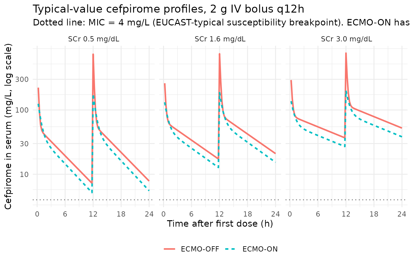
Stochastic VPC
sim_stoch |>
  dplyr::filter(time > 0, !is.na(Cc)) |>
  dplyr::group_by(scr, ecmo, time) |>
  dplyr::summarise(
    Q05 = stats::quantile(Cc, 0.05, na.rm = TRUE),
    Q50 = stats::quantile(Cc, 0.50, na.rm = TRUE),
    Q95 = stats::quantile(Cc, 0.95, na.rm = TRUE),
    .groups = "drop"
  ) |>
  dplyr::mutate(
    scr_lbl  = factor(sprintf("SCr %.1f mg/dL", scr),
                      levels = sprintf("SCr %.1f mg/dL", scr_levels)),
    ecmo_lbl = ifelse(ecmo == 1L, "ECMO-ON", "ECMO-OFF")
  ) |>
  ggplot(aes(time, Q50, colour = ecmo_lbl, fill = ecmo_lbl)) +
  geom_ribbon(aes(ymin = Q05, ymax = Q95),
              alpha = 0.25, colour = NA) +
  geom_line(linewidth = 0.9) +
  geom_hline(yintercept = 4, linetype = "dotted", colour = "grey40") +
  facet_wrap(~scr_lbl) +
  scale_y_log10() +
  scale_x_continuous(breaks = seq(0, sim_end_h, 6)) +
  labs(
    x = "Time after first dose (h)",
    y = "Cefpirome in serum (mg/L, log scale)",
    colour   = NULL,
    fill     = NULL,
    title    = "Stochastic VPC, 2 g IV bolus q12h, by SCr and ECMO state",
    subtitle = "Median and 5-95 percentile band (50 simulated subjects per stratum). Dotted: MIC = 4 mg/L."
  ) +
  theme_minimal() +
  theme(legend.position = "bottom")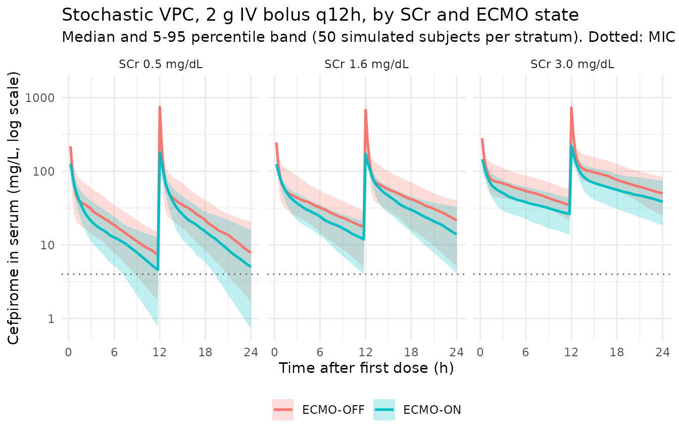
Probability of target attainment (Figure 2 / Table S2 replication)
Kang 2020 used a 65% fT > MIC target for cefpirome (Methods,
Simulations; following Mouton 2002 and Roberts 2011). The simulation
framework below follows the paper’s approach: stochastic simulation
across the SCr x ECMO strata, then per-subject computation of the
fraction of the 24-h observation interval spent above each candidate
MIC. Protein binding of 10% is applied (Methods: “when a protein
binding constant of 10% was applied”), so the unbound concentration
is Cc_free = 0.9 * Cc. PTA is the fraction of subjects
achieving fT > MIC >= 65% over the 12-24 h window (the second q12h
dosing interval).
mic_grid <- c(0.5, 1, 2, 4, 8, 16, 32)

pta_subject <- function(time, Cc_free, mic, t0, t1) {
  keep <- which(time >= t0 & time <= t1)
  if (length(keep) < 2) return(NA_real_)
  t  <- time[keep]
  cf <- Cc_free[keep]
  above <- cf > mic
  sum(diff(t) * ((above[-length(above)] + above[-1]) / 2)) / (t1 - t0)
}

pta_long <- sim_stoch |>
  dplyr::filter(!is.na(Cc)) |>
  dplyr::mutate(Cc_free = 0.9 * Cc) |>
  dplyr::arrange(scr, ecmo, id, time)

pta_per_subject <- pta_long |>
  dplyr::group_by(scr, ecmo, id) |>
  dplyr::group_modify(function(df, key) {
    fT <- vapply(mic_grid,
                 function(mic) pta_subject(df$time, df$Cc_free, mic, 12, 24),
                 numeric(1))
    tibble::tibble(mic = mic_grid, fT_above = fT)
  }) |>
  dplyr::ungroup()

pta_tab <- pta_per_subject |>
  dplyr::group_by(scr, ecmo, mic) |>
  dplyr::summarise(pta = mean(fT_above >= 0.65, na.rm = TRUE),
                   .groups = "drop")

pta_tab |>
  dplyr::mutate(
    scr_lbl  = factor(sprintf("SCr %.1f mg/dL", scr),
                      levels = sprintf("SCr %.1f mg/dL", scr_levels)),
    ecmo_lbl = ifelse(ecmo == 1L, "ECMO-ON", "ECMO-OFF")
  ) |>
  ggplot(aes(mic, pta, colour = ecmo_lbl, linetype = ecmo_lbl)) +
  geom_line(linewidth = 0.9) +
  geom_point(size = 1.8) +
  geom_hline(yintercept = 0.9, linetype = "dashed", colour = "grey40") +
  facet_wrap(~scr_lbl) +
  scale_x_log10(breaks = mic_grid) +
  scale_y_continuous(labels = scales::percent_format(accuracy = 1),
                     limits = c(0, 1)) +
  labs(
    x = "MIC (mg/L, log scale)",
    y = "Probability of target attainment (fT > MIC >= 65%)",
    colour   = NULL,
    linetype = NULL,
    title    = "Figure 2 / Table S2 replication: PTA vs MIC, by SCr x ECMO",
    subtitle = "2 g IV bolus q12h; PTA computed over the second dosing interval (12-24 h). Dashed: 90% PTA threshold."
  ) +
  theme_minimal() +
  theme(legend.position = "bottom")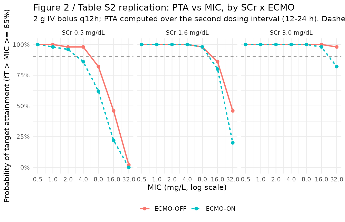
PKNCA on the simulated cohort
PKNCA computes per-interval Cmax, Tmax and AUC over the first dosing interval (0-12 h after the loading 2 g IV bolus). The simulated values below serve as an internal sanity check that the simulation produces NCA values in the clinically expected range. Kang 2020’s individual NCA-type summaries (Cmax, Tmax, half-life per patient) live in supplemental Table S1, which is not on disk; see the Assumptions and deviations section for the per-publication NCA cross-check status.
first_interval_h <- 12

# Ensure a time-zero observation row per subject for clean AUC integration.
zero_row <- sim_stoch |>
  dplyr::distinct(cohort, scr, ecmo, id) |>
  dplyr::mutate(time = 0, Cc = 0)

sim_for_nca <- dplyr::bind_rows(
  zero_row,
  sim_stoch |>
    dplyr::filter(!is.na(Cc), time > 0, time <= first_interval_h) |>
    dplyr::select(cohort, scr, ecmo, id, time, Cc)
) |>
  dplyr::mutate(treatment = sprintf("SCr %.1f, %s",
                                    scr,
                                    ifelse(ecmo == 1L, "ECMO-ON",
                                                       "ECMO-OFF"))) |>
  dplyr::filter(!is.na(Cc)) |>
  dplyr::arrange(treatment, id, time) |>
  as.data.frame()

doses_for_nca <- events |>
  dplyr::filter(evid == 1L, time == 0) |>
  dplyr::mutate(treatment = sprintf("SCr %.1f, %s",
                                    scr,
                                    ifelse(ecmo == 1L, "ECMO-ON",
                                                       "ECMO-OFF"))) |>
  dplyr::select(id, time, amt, treatment) |>
  as.data.frame()

conc_obj <- PKNCA::PKNCAconc(
  data    = sim_for_nca,
  formula = Cc ~ time | treatment + id,
  concu   = "mg/L",
  timeu   = "hr"
)
dose_obj <- PKNCA::PKNCAdose(
  data    = doses_for_nca,
  formula = amt ~ time | treatment + id,
  doseu   = "mg"
)

intervals <- data.frame(
  start         = 0,
  end           = c(first_interval_h, Inf),
  cmax          = c(TRUE,  FALSE),
  tmax          = c(TRUE,  FALSE),
  auclast       = c(TRUE,  FALSE),
  aucinf.obs    = c(FALSE, TRUE),
  half.life     = c(FALSE, TRUE)
)

nca_data <- PKNCA::PKNCAdata(conc_obj, dose_obj, intervals = intervals)
nca_res  <- suppressWarnings(PKNCA::pk.nca(nca_data))

knitr::kable(
  summary(nca_res),
  caption = "Simulated NCA parameters by SCr x ECMO stratum (first 2 g IV bolus, q12h regimen)."
)| Interval Start | Interval End | treatment | N | AUClast (hr*mg/L) | Cmax (mg/L) | Tmax (hr) | Half-life (hr) | AUCinf,obs (hr*mg/L) |
|---|---|---|---|---|---|---|---|---|
| 0 | 12 | SCr 0.5, ECMO-OFF | 50 | 406 [29.4] | 706 [35.7] | 12.0 [12.0, 12.0] | . | . |
| 0 | Inf | SCr 0.5, ECMO-OFF | 50 | . | . | . | NC | NC |
| 0 | 12 | SCr 0.5, ECMO-ON | 50 | 263 [27.5] | 182 [39.6] | 12.0 [12.0, 12.0] | . | . |
| 0 | Inf | SCr 0.5, ECMO-ON | 50 | . | . | . | NC | NC |
| 0 | 12 | SCr 1.6, ECMO-OFF | 50 | 557 [29.0] | 714 [34.3] | 12.0 [12.0, 12.0] | . | . |
| 0 | Inf | SCr 1.6, ECMO-OFF | 50 | . | . | . | NC | NC |
| 0 | 12 | SCr 1.6, ECMO-ON | 50 | 390 [19.9] | 189 [34.3] | 12.0 [12.0, 12.0] | . | . |
| 0 | Inf | SCr 1.6, ECMO-ON | 50 | . | . | . | NC | NC |
| 0 | 12 | SCr 3.0, ECMO-OFF | 50 | 833 [21.6] | 731 [36.8] | 12.0 [12.0, 12.0] | . | . |
| 0 | Inf | SCr 3.0, ECMO-OFF | 50 | . | . | . | NC | NC |
| 0 | 12 | SCr 3.0, ECMO-ON | 50 | 559 [24.3] | 212 [28.8] | 12.0 [12.0, 12.0] | . | . |
| 0 | Inf | SCr 3.0, ECMO-ON | 50 | . | . | . | NC | NC |
Comparison against published values
Kang 2020 reports no main-text NCA table. The principal cross-checks available against the printed paper are:
CL at SCr = 1.6 mg/dL. Kang 2020 Results states 3.92 L/h (ECMO-ON) and 2.78 L/h (ECMO-OFF). The packaged model reproduces both exactly (see typical-value table above). These were the only published numerical cross-checks of the final-model covariate equations.
PTA shape vs. SCr. Kang 2020 Results: “the simulations showed that patients with low SCr during ECMO-ON had lower PTA than patients with high SCr during ECMO-OFF; so, a higher dosage of cefpirome was required.” The Figure 2 / Table S2 replication above reproduces this qualitatively – the SCr-0.5 / ECMO-ON facet has the leftmost PTA curve drop, the SCr-3.0 / ECMO-OFF facet the rightmost, with SCr-1.6 spanning the two. The model fits the same observed Severance cohort, so the PTA agreement is corroborative rather than independent.
2 g q8h IV bolus recommended for normal renal function on ECMO. Kang 2020 Abstract / Conclusions: “Cefpirome of 2 g every 8 h for intravenous bolus injection or 2 g every 12 h for extended infusion over 4 h was recommended with normal kidney function receiving ECMO.” At SCr = 1.6 mg/dL on ECMO, the 2 g q12h IV bolus regimen simulated here drops below the 90% PTA dashed line between MIC 1 and MIC 2 mg/L, consistent with the paper’s conclusion that the 2 g q12h regimen is inadequate for ECMO patients and a q8h interval is needed for higher MIC bacteria (EUCAST cefpirome susceptibility cutoff for Enterobacterales is 4 mg/L).
Assumptions and deviations
In-equation reference value 1.6 mg/dL is not the cohort median. Table 1 reports a cohort median SCr of 1.58 mg/dL during ECMO and 1.84 mg/dL after weaning. The paper’s printed covariate equation uses 1.6 mg/dL as the in-exponent centering point, which rounds the on-ECMO median to one decimal. This rounding does not change the parameter point estimate but means the typical-value CL evaluated exactly at SCr = 1.6 (rather than at SCr = 1.58 or 1.84) is the published reference. The packaged model uses 1.6 mg/dL as printed.
Power-form CL covariate with SCr in the exponent. Most popPK CL covariate equations on a renal-function variable have the variable in the base of a power (e.g.
(CRCL / ref)^exponent). Kang 2020 chose the opposite: a constant base (0.487) raised to an SCr-dependent exponent (SCr / 1.6). At SCr = 0 the multiplier evaluates to 1 (solcl = log(5.71)is the SCr-= 0 anchor, not a physiological reference value); at SCr = 1.6 the multiplier evaluates to 0.487 and the ECMO-OFF CL equals 5.71 * 0.487 = 2.78 L/h. The packaged model uses the equation as printed.Diagonal IIV. Kang 2020 Table 2 reports one CV per parameter (CL 35.1%, V1 37.4%, V2 47.5%) and no covariances. Methods (Base model development) describes an exponential variance model on eta but does not state whether off-diagonal OMEGA terms were estimated. The packaged model uses diagonal IIV (no eta correlations). The paper’s Results states “We checked the interindividual variability (ETA) correlation plot for the final PK model, but it has not shown any trends,” which is consistent with diagonal IIV being adequate.
omega^2 = log(CV^2 + 1). Table 2 reports IIV as CV%; the corresponding log-normal variance was computed viaomega^2 = log(CV^2 + 1)(the standard log-normal back-transform) and entered as theeta...initial value. CL: log(0.351^2 + 1) = 0.11618; V1: log(0.374^2 + 1) = 0.13092; V2: log(0.475^2 + 1) = 0.20345.Proportional residual error. Kang 2020 Results: “The residual variability was best described by a proportional residual error model.” Table 2 reports 21.7% CV. Encoded as
propSd = 0.217(the proportional SD fraction in linear DV space).Supplemental Table S1 (individual NCA) not on disk. The paper references S1 for per-patient half-life, Cmax, and Tmax. The supplement was not obtainable through the EuropePMC / PMC / ASM endpoints attempted during extraction (the EuropePMC PDF-render endpoint returned the main PDF only; the journals.asm.org supplement URL returned HTML rather than the PDF). The packaged model’s parameters all come from main-text Table 2 and the printed equations in Results; the missing supplement contains derived NCA-type values rather than estimated model parameters, so the absence does not affect the model. The simulated NCA values in the PKNCA section are internal sanity checks; no per-patient comparison against the published S1 is performed.
Time-varying CREAT and ECMO_STATUS. Kang 2020 Methods (Covariate model development): “All data were recorded during sampling and tested as time-varying covariates.” Both
CREATandECMO_STATUSare time-varying within subject. The vignette’s simulation cohort fixes both covariates within a subject so each subject occupies one of the six SCr x ECMO strata for the entire observation window; this is a simplification appropriate for a clean PTA visualization but differs from the patient-trajectory reality in the source cohort, where ECMO_STATUS flips from 1 to 0 at decannulation and SCr drifts over a multi-day ECMO run.VA-ECMO only. The Kang 2020 cohort comprises VA-ECMO patients exclusively (Methods, Subjects: “Eligible patients were 19 years of age or older, receiving venoarterial ECMO (VA-ECMO)”). The model’s
ECMO_STATUSbinary covariate does not distinguish VA-ECMO from VV-ECMO; users transferring this model to a VV-ECMO cohort should be aware that the magnitude of the V1 expansion (4.22-fold) reflects circuit volume and hemodynamic state that may differ between VA- and VV-ECMO.CRRT not modelled. Five of 15 patients received CRRT during ECMO. CRRT was screened during stepwise selection and dropped from the final model (Kang 2020 Discussion: “the use of CRRT was dropped out through stepwise covariate modeling having larger OFV than SCr or ECMO”). The packaged model does not include a CRRT indicator; for a CRRT-on cohort, users should consult the Shekar 2014 meropenem model (
Shekar_2014_meropenem.R) for an analogous beta-lactam CRRT covariate structure.Race / ethnicity not reported. Table 1 does not include race; the single-centre Severance Hospital cohort is presumed predominantly Korean. No race effect is modelled.
Protein binding for PTA. The Methods state cefpirome protein binding is 10% (Methods, Simulations: “when a protein binding constant of 10% was applied”); the unbound concentration is
Cc_free = 0.9 * Cc. The 10% binding is treated as a fixed average; no binding-saturation submodel is included.