Methotrexate nanoparticles and nanoemulsions in rats (Jeong 2021)
Source:vignettes/articles/Jeong_2021_methotrexate_nanoformulations.Rmd
Jeong_2021_methotrexate_nanoformulations.RmdModel and source
Jeong 2021 reanalysed the plasma data of two earlier rat formulation studies from the same group (methotrexate-loaded PLGA nanoparticles, Jang 2019; methotrexate-loaded olive-oil/Labrasol nanoemulsions, Jang 2020) with Phoenix NLME. The paper reports two final population PK models, each fitted to its own data set, and both are packaged here:
Jeong_2021_methotrexate_nanoformulation_rat– free methotrexate solution versus any nanoformulation (Section 3.2, Equations (1)-(5), Table 3), fitted to all 40 rats.Jeong_2021_methotrexate_nanoemulsion_rat– PLGA nanoparticles versus nanoemulsions (Section 3.4, Equations (6)-(10), Table 9), fitted to the 20 rats that received a nanoformulation.Citation: Jeong S-H, Jang J-H, Lee Y-B. Pharmacokinetic Comparison between Methotrexate-Loaded Nanoparticles and Nanoemulsions as Hard- and Soft-Type Nanoformulations: A Population Pharmacokinetic Modeling Approach. Pharmaceutics. 2021;13(7):1050. doi:10.3390/pharmaceutics13071050
Article: Pharmaceutics 2021;13(7):1050. https://doi.org/10.3390/pharmaceutics13071050
Both models are one-compartment with first-order absorption and
elimination, oral bioavailability, exponential IIV and a log-additive
residual error. The formulation indicator enters every covariate
relationship as a linear deviation,
P = tvP * (1 + dPdFormulation * indicator) * exp(eta).
Population
Male Sprague-Dawley rats, 7-9 weeks old and 240-260 g, without disease (Jeong 2021 Section 2.1). Each rat received one single dose by one route, with 5 rats per arm:
| Arm | Oral dose | IV dose | Source study |
|---|---|---|---|
| Free methotrexate solution | 5 mg/kg | 5 mg/kg | PLGA nanoparticle study (Figure 1) |
| Free methotrexate solution | 0.06 mg/kg | 0.024 mg/kg | Nanoemulsion study (Figure 2) |
| PLGA nanoparticles | 5 mg/kg | 5 mg/kg | Table 6 |
| Olive-oil/Labrasol nanoemulsions | 0.06 mg/kg | 0.024 mg/kg | Table 6 |
The two models’ population metadata carry the same
information
(readModelDb("Jeong_2021_methotrexate_nanoemulsion_rat")$population).
Source trace
| Equation / parameter | Free-vs-nano model | NP-vs-NE model | Source location |
|---|---|---|---|
| Structure: 1-cmt, first-order absorption, IV into central | – | – | Section 3.2 and 3.4; Figure 7 |
| Formulation effects as linear deviation | Eq. (1), (2), (4), (5) | Eq. (6), (7), (9), (10) | Sections 3.2, 3.4 |
lvc (tvV) |
14.889 L/kg | 18.832 L/kg | Table 3 / Table 9 |
lcl (tvCL) |
14.577 L/h/kg | 9.167 L/h/kg | Table 3 / Table 9 |
lka (tvKa) |
0.582 1/h | 0.714 1/h | Table 3 / Table 9 |
lfdepot (tvF) |
0.272 | 0.334 | Table 3 / Table 9 |
e_form_*_vc (dVdFormulation) |
0.429 | -0.986 | Table 3 / Table 9 |
e_form_*_cl (dCLdFormulation) |
-0.355 | -0.990 | Table 3 / Table 9 |
e_form_*_ka (dKadFormulation) |
10.883 | 1.552 | Table 3 / Table 9 |
e_form_*_fdepot (dFdFormulation) |
4.246 | 0.193 | Table 3 / Table 9 |
etalvc |
6.3504e-6 (IIV 0.252%) | 5.6644e-6 (IIV 0.238%) | Table 3 / Table 9 IIV (%) column |
etalcl |
0.338 | 0.0084622 (IIV 9.199%) | Table 3 omega^2 / Table 9 IIV (%) column |
etalka |
4e-10 (IIV 0.002%) | 4e-10 (IIV 0.002%) | Table 3 / Table 9 IIV (%) column |
etalfdepot |
0.386 | 0.0010278 (IIV 3.206%) | Table 3 omega^2 / Table 9 IIV (%) column |
expSd (sigma, log-additive) |
1.269 | 0.552 | Table 3 / Table 9 |
| Absorption lag time (omitted) | tvTlag 0.000 h | tvTlag 0.000 h | Table 3 / Table 9, Eq. (3) / (8) |
Virtual cohorts
Each arm of the source studies is simulated with 100 virtual rats. Doses are per kg, so no body weight is needed. The sampling grid follows the concentration-time profiles in Figure 4 (0.25-12 h), with a time-zero record added for NCA.
obs_times <- c(0, 0.25, 0.5, 0.75, 1, 2, 4, 6, 8, 12)
n_per_arm <- 100L

arms_ne <- tribble(
  ~arm,                    ~formulation,     ~admin,  ~dose_mgkg,~FORM_MTX_NANOEMULSION,
  "NP oral 5 mg/kg",       "Nanoparticles",  "oral",  5,      0L,
  "NP IV 5 mg/kg",         "Nanoparticles",  "iv",    5,      0L,
  "NE oral 0.06 mg/kg",    "Nanoemulsions",  "oral",  0.06,   1L,
  "NE IV 0.024 mg/kg",     "Nanoemulsions",  "iv",    0.024,  1L
)

arms_nano <- tribble(
  ~arm,                    ~formulation,     ~admin,  ~dose_mgkg,~FORM_MTX_NANO,
  "Free oral 5 mg/kg",     "Free solution",  "oral",  5,      0L,
  "Free IV 5 mg/kg",       "Free solution",  "iv",    5,      0L,
  "Free oral 0.06 mg/kg",  "Free solution",  "oral",  0.06,   0L,
  "Free IV 0.024 mg/kg",   "Free solution",  "iv",    0.024,  0L,
  "NP oral 5 mg/kg",       "Nanoparticles",  "oral",  5,      1L,
  "NP IV 5 mg/kg",         "Nanoparticles",  "iv",    5,      1L,
  "NE oral 0.06 mg/kg",    "Nanoemulsions",  "oral",  0.06,   1L,
  "NE IV 0.024 mg/kg",     "Nanoemulsions",  "iv",    0.024,  1L
)

# One oral dose into depot or one IV bolus into central per rat, then
# observation records on the central state (Cc is computed from it).
make_events <- function(arms, n, times) {
  subj <- arms |>
    mutate(arm_idx = row_number()) |>
    tidyr::crossing(rep = seq_len(n)) |>
    mutate(id = (arm_idx - 1L) * n + rep)
  doses <- subj |>
    mutate(time = 0, amt = dose_mgkg, evid = 1L,
           cmt = if_else(admin == "oral", "depot", "central"))
  obs <- subj |>
    tidyr::crossing(time = times) |>
    mutate(amt = NA_real_, evid = 0L, cmt = "central")
  bind_rows(doses, obs) |>
    select(-arm_idx, -rep) |>
    arrange(id, time, desc(evid)) |>
    as.data.frame()
}

ev_ne <- make_events(arms_ne, n_per_arm, obs_times)
ev_nano <- make_events(arms_nano, n_per_arm, obs_times)
stopifnot(
  length(unique(ev_ne$id)) == nrow(arms_ne) * n_per_arm,
  length(unique(ev_nano$id)) == nrow(arms_nano) * n_per_arm
)
Simulation
mod_ne <- rxode2::rxode2(readModelDb("Jeong_2021_methotrexate_nanoemulsion_rat"))
#> ℹ parameter labels from comments will be replaced by 'label()'
mod_nano <- rxode2::rxode2(readModelDb("Jeong_2021_methotrexate_nanoformulation_rat"))
#> ℹ parameter labels from comments will be replaced by 'label()'

keep_cols <- c("arm", "formulation", "admin", "dose_mgkg")

# The states are amounts in mg/kg, and the low-dose arms fall to about
# 1e-10 mg/kg by 12 h, below the default absolute tolerance. Tight
# tolerances stop solver noise from producing negative concentrations.
tol <- list(atol = 1e-14, rtol = 1e-10)

rxode2::rxSetSeed(20210709L)
sim_ne <- rxode2::rxSolve(mod_ne, events = ev_ne, keep = keep_cols,
                          atol = tol$atol, rtol = tol$rtol) |>
  as.data.frame()
rxode2::rxSetSeed(20210710L)
sim_nano <- rxode2::rxSolve(mod_nano, events = ev_nano, keep = keep_cols,
                            atol = tol$atol, rtol = tol$rtol) |>
  as.data.frame()
# A few fast-clearing virtual rats still undershoot zero by ~1e-15 ng/mL at
# 8-12 h. Assert that this is noise relative to the peak, then floor it so
# PKNCA does not take logs of negative values.
stopifnot(min(sim_ne$Cc) >= -1e-9 * max(sim_ne$Cc),
          min(sim_nano$Cc) >= -1e-9 * max(sim_nano$Cc))
sim_ne$Cc <- pmax(sim_ne$Cc, 0)
sim_nano$Cc <- pmax(sim_nano$Cc, 0)

# Typical-value (no IIV, no residual) solves on a dense grid for the
# figure replicates and the closed-form check. zeroRe() leaves no omega,
# which rxode2 reports with a warning for a multi-subject event table.
dense_times <- sort(unique(c(seq(0, 12, by = 0.05), obs_times)))
typ_ne <- suppressWarnings(rxode2::rxSolve(
  rxode2::zeroRe(mod_ne),
  events = make_events(arms_ne, 1L, dense_times), keep = keep_cols,
  atol = tol$atol, rtol = tol$rtol
)) |> as.data.frame()
#> ℹ omega/sigma items treated as zero: 'etalvc', 'etalcl', 'etalka', 'etalfdepot'
typ_nano <- suppressWarnings(rxode2::rxSolve(
  rxode2::zeroRe(mod_nano),
  events = make_events(arms_nano, 1L, dense_times), keep = keep_cols,
  atol = tol$atol, rtol = tol$rtol
)) |> as.data.frame()
#> ℹ omega/sigma items treated as zero: 'etalvc', 'etalcl', 'etalka', 'etalfdepot'
Closed-form check of the encoding
A one-compartment model with first-order absorption has an analytic solution, so the typical-value solve must reproduce it for every arm. This check shares its parameters with the solve, so any difference is numerical error and a tight bound is appropriate. It pins the per-kg units (x 1000 to ng/mL), the formulation coefficients on V, CL, ka and F, and the dosing compartments.
closed_form <- function(arms, tv, indicator) {
  arms |>
    mutate(
      v = tv$v * (1 + tv$e_v * .data[[indicator]]),
      cl = tv$cl * (1 + tv$e_cl * .data[[indicator]]),
      ka = tv$ka * (1 + tv$e_ka * .data[[indicator]]),
      f = tv$f * (1 + tv$e_f * .data[[indicator]]),
      kel = cl / v
    ) |>
    select(arm, admin, dose_mgkg, v, cl, ka, f, kel)
}

tv_ne <- list(v = 18.832, cl = 9.167, ka = 0.714, f = 0.334,
              e_v = -0.986, e_cl = -0.990, e_ka = 1.552, e_f = 0.193)
tv_nano <- list(v = 14.889, cl = 14.577, ka = 0.582, f = 0.272,
                e_v = 0.429, e_cl = -0.355, e_ka = 10.883, e_f = 4.246)

check_closed_form <- function(typ, params) {
  typ |>
    select(arm, time, Cc) |>
    inner_join(params, by = "arm") |>
    mutate(
      Cc_exact = if_else(
        admin == "iv",
        1000 * dose_mgkg / v * exp(-kel * time),
        1000 * f * dose_mgkg * ka / (v * (ka - kel)) * (exp(-kel * time) - exp(-ka * time))
      ),
      rel_err = abs(Cc - Cc_exact) / max(Cc_exact)
    ) |>
    group_by(arm) |>
    summarise(max_rel_err = max(rel_err), .groups = "drop")
}

cf_ne <- check_closed_form(typ_ne, closed_form(arms_ne, tv_ne, "FORM_MTX_NANOEMULSION"))
cf_nano <- check_closed_form(typ_nano, closed_form(arms_nano, tv_nano, "FORM_MTX_NANO"))
knitr::kable(bind_rows(
  mutate(cf_ne, model = "NP-vs-NE"),
  mutate(cf_nano, model = "Free-vs-nano")
) |> select(model, arm, max_rel_err), digits = 8,
caption = "Largest relative difference between the typical-value solve and the analytic one-compartment solution (scaled by each arm's peak).")| model | arm | max_rel_err |
|---|---|---|
| NP-vs-NE | NE IV 0.024 mg/kg | 0 |
| NP-vs-NE | NE oral 0.06 mg/kg | 0 |
| NP-vs-NE | NP IV 5 mg/kg | 0 |
| NP-vs-NE | NP oral 5 mg/kg | 0 |
| Free-vs-nano | Free IV 0.024 mg/kg | 0 |
| Free-vs-nano | Free IV 5 mg/kg | 0 |
| Free-vs-nano | Free oral 0.06 mg/kg | 0 |
| Free-vs-nano | Free oral 5 mg/kg | 0 |
| Free-vs-nano | NE IV 0.024 mg/kg | 0 |
| Free-vs-nano | NE oral 0.06 mg/kg | 0 |
| Free-vs-nano | NP IV 5 mg/kg | 0 |
| Free-vs-nano | NP oral 5 mg/kg | 0 |
Replicate published figures
Figure 4 – dose-normalised profiles, nanoparticles vs nanoemulsions
Figure 4 plots the mean dose-normalised concentration (ng/mL per mg/kg) of the two nanoformulations after oral (A) and intravenous (B) dosing. The published means run roughly 6 ng/mL per mg/kg at the nanoparticle oral peak versus about 1400 for the nanoemulsions, and about 140 versus 7500 at 0.25 h after IV dosing (Table 6 Cmax/Dose).
typ_ne |>
  filter(time > 0) |>
  mutate(Cc_dn = Cc / dose_mgkg,
         route_label = if_else(admin == "oral", "Oral", "Intravenous")) |>
  ggplot(aes(time, Cc_dn, colour = formulation)) +
  geom_line(linewidth = 0.8) +
  facet_wrap(~route_label) +
  scale_y_log10() +
  labs(x = "Time (h)", y = "Dose-normalised Cc (ng/mL per mg/kg)",
       colour = NULL)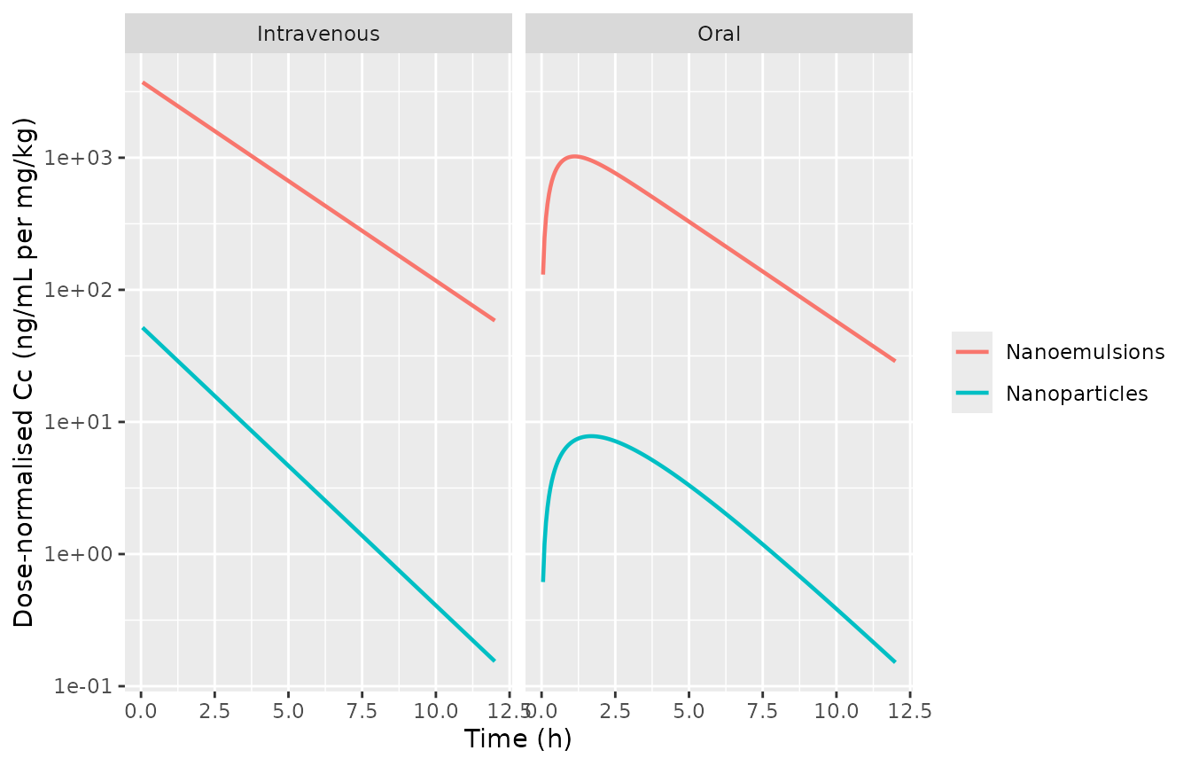
Replicates Figure 4 of Jeong 2021 with the nanoparticle-vs-nanoemulsion model: typical-value dose-normalised methotrexate concentration after oral (left) and IV (right) dosing.
The model reproduces the direction and the roughly 100- to 200-fold separation between the formulations. It does not reproduce the early IV peak (for example, the nanoparticle C0 of 1344.57 ng/mL in Table 6 against a model-predicted 265 ng/mL). A one-compartment model cannot represent the rapid initial decline of an IV profile. The authors state that two- and three-compartment models “could not be applied to multiple subjects”.
Figure 9 – visual predictive check by formulation
expSd_ne <- rxode2::rxode(mod_ne)$theta[["expSd"]]
set.seed(20210711L)
vpc_ne <- sim_ne |>
  filter(time > 0) |>
  mutate(obs = Cc * exp(expSd_ne * rnorm(n()))) |>
  group_by(formulation, time) |>
  summarise(q05 = quantile(obs, 0.05), q50 = median(obs), q95 = quantile(obs, 0.95),
            .groups = "drop")

ggplot(vpc_ne, aes(time)) +
  geom_ribbon(aes(ymin = q05, ymax = q95), fill = "steelblue", alpha = 0.25) +
  geom_line(aes(y = q50), colour = "steelblue4", linewidth = 0.8) +
  facet_wrap(~formulation) +
  scale_y_log10() +
  labs(x = "Time (h)", y = "Plasma methotrexate (ng/mL)")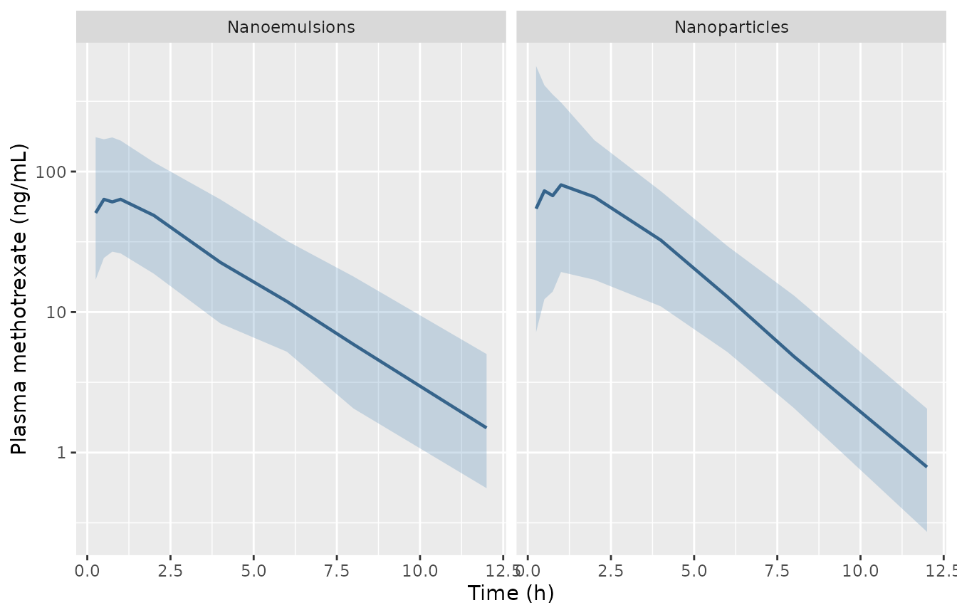
Replicates Figure 9 of Jeong 2021: simulated 5th, 50th and 95th percentiles of plasma methotrexate for the nanoparticle-vs-nanoemulsion model, pooled over oral and IV dosing within each formulation, with residual error added.
Figure 9 plots concentrations on a natural-log axis. The nanoparticle panel runs from about e^6.5 ng/mL at 0.25 h (the IV arm) down to about e^0 to e^1.5 at 12 h. The nanoemulsion panel runs from about e^4 to e^5 early down to about e^0 to e^1 at 12 h. In the simulation the nanoparticle 95th percentile is e^6.3 at 0.25 h and the 12 h median is e^-0.2. For the nanoemulsions the 0.25 h median is e^3.9 and the 12 h median is e^0.4, the same ranges as the published panels.
PKNCA validation
run_nca <- function(sim, events) {
  conc <- sim |>
    filter(!is.na(Cc)) |>
    select(id, time, Cc, arm)
  dose_df <- events |>
    filter(evid == 1L) |>
    select(id, time, amt, arm)
  intervals <- data.frame(
    start = 0, end = Inf,
    cmax = TRUE, tmax = TRUE, auclast = TRUE, aucinf.obs = TRUE,
    half.life = TRUE
  )
  PKNCA::pk.nca(PKNCA::PKNCAdata(
    PKNCA::PKNCAconc(conc, Cc ~ time | arm + id),
    PKNCA::PKNCAdose(dose_df, amt ~ time | arm + id),
    intervals = intervals
  ))
}

nca_ne <- run_nca(sim_ne, ev_ne)
nca_nano <- run_nca(sim_nano, ev_nano)
Comparison against published NCA
Table 6 gives the NCA of the nanoformulation arms (mean of 5 rats). The free-solution arms are shown only as bar charts in Figures 1 and 2; the values below for those arms were read off the bar heights by the maintainers and are approximate. The simulated values are medians of 100 virtual rats per arm. Cmax is compared for the oral arms only. For IV bolus doses the paper’s Cmax is the first sample (0.25 h), which a one-compartment model does not represent (see Figure 4 above).
ref_table6 <- tribble(
  ~arm,                  ~PPTESTCD,     ~PPORRES,
  "NP oral 5 mg/kg",     "cmax",        31.19,
  "NP oral 5 mg/kg",     "tmax",        0.92,
  "NP oral 5 mg/kg",     "auclast",     142.05,
  "NP oral 5 mg/kg",     "aucinf.obs",  148.44,
  "NP oral 5 mg/kg",     "half.life",   2.59,
  "NE oral 0.06 mg/kg",  "cmax",        81.72,
  "NE oral 0.06 mg/kg",  "tmax",        1.35,
  "NE oral 0.06 mg/kg",  "auclast",     288.35,
  "NE oral 0.06 mg/kg",  "aucinf.obs",  291.34,
  "NE oral 0.06 mg/kg",  "half.life",   1.58,
  "NP IV 5 mg/kg",       "auclast",     720.15,
  "NP IV 5 mg/kg",       "aucinf.obs",  722.53,
  "NP IV 5 mg/kg",       "half.life",   1.62,
  "NE IV 0.024 mg/kg",   "auclast",     268.94,
  "NE IV 0.024 mg/kg",   "aucinf.obs",  300.56,
  "NE IV 0.024 mg/kg",   "half.life",   6.38
)

# Approximate values read off Figure 1 (free solution, 5 mg/kg) and Figure 2
# (free solution, 0.06 mg/kg oral / 0.024 mg/kg IV) by the maintainers.
ref_fig12 <- tribble(
  ~arm,                    ~PPTESTCD,     ~PPORRES,
  "Free oral 5 mg/kg",     "cmax",        17,
  "Free oral 5 mg/kg",     "aucinf.obs",  62,
  "Free oral 5 mg/kg",     "half.life",   1.55,
  "Free IV 5 mg/kg",       "aucinf.obs",  378,
  "Free IV 5 mg/kg",       "half.life",   1.6,
  "Free oral 0.06 mg/kg",  "cmax",        12,
  "Free oral 0.06 mg/kg",  "aucinf.obs",  29,
  "Free oral 0.06 mg/kg",  "half.life",   1.1,
  "Free IV 0.024 mg/kg",   "aucinf.obs",  94,
  "Free IV 0.024 mg/kg",   "half.life",   0.85
)

nca_units <- c(cmax = "ng/mL", tmax = "h", auclast = "ng*h/mL",
               aucinf.obs = "ng*h/mL", half.life = "h")
Nanoparticle-vs-nanoemulsion model
cmp_ne <- nlmixr2lib::ncaComparisonTable(
  simulated = nca_ne, reference = ref_table6, by = "arm",
  units = nca_units, tolerance_pct = 20
)
knitr::kable(cmp_ne, caption = "Nanoparticle-vs-nanoemulsion model: simulated median vs Jeong 2021 Table 6. * differs from the reference by more than 20%.")| NCA parameter | arm | Reference | Simulated | % diff |
|---|---|---|---|---|
| Cmax (ng/mL) | NP oral 5 mg/kg | 31.2 | 38.4 | +23.2%* |
| Cmax (ng/mL) | NE oral 0.06 mg/kg | 81.7 | 61.4 | -24.9%* |
| Tmax (h) | NP oral 5 mg/kg | 0.92 | 2 | +117.4%* |
| Tmax (h) | NE oral 0.06 mg/kg | 1.35 | 1 | -25.9%* |
| AUC0-∞ (obs) (ng*h/mL) | NP oral 5 mg/kg | 148 | 178 | +19.8% |
| AUC0-∞ (obs) (ng*h/mL) | NE oral 0.06 mg/kg | 291 | 260 | -10.8% |
| AUC0-∞ (obs) (ng*h/mL) | NP IV 5 mg/kg | 723 | 545 | -24.5%* |
| AUC0-∞ (obs) (ng*h/mL) | NE IV 0.024 mg/kg | 301 | 259 | -13.8% |
| AUClast (ng*h/mL) | NP oral 5 mg/kg | 142 | 176 | +23.9%* |
| AUClast (ng*h/mL) | NE oral 0.06 mg/kg | 288 | 255 | -11.7% |
| AUClast (ng*h/mL) | NP IV 5 mg/kg | 720 | 544 | -24.5%* |
| AUClast (ng*h/mL) | NE IV 0.024 mg/kg | 269 | 255 | -5.1% |
| t½ (h) | NP oral 5 mg/kg | 2.59 | 1.54 | -40.6%* |
| t½ (h) | NE oral 0.06 mg/kg | 1.58 | 2.01 | +27.1%* |
| t½ (h) | NP IV 5 mg/kg | 1.62 | 1.42 | -12.3% |
| t½ (h) | NE IV 0.024 mg/kg | 6.38 | 1.97 | -69.1%* |
Free-solution-vs-nanoformulation model
cmp_nano <- nlmixr2lib::ncaComparisonTable(
  simulated = nca_nano, reference = bind_rows(ref_fig12, ref_table6), by = "arm",
  units = nca_units, tolerance_pct = 20
)
knitr::kable(cmp_nano, caption = "Free-solution-vs-nanoformulation model: simulated median vs Jeong 2021 Figures 1-2 (free solution, approximate) and Table 6 (nanoformulations). * differs from the reference by more than 20%.")| NCA parameter | arm | Reference | Simulated | % diff |
|---|---|---|---|---|
| Cmax (ng/mL) | Free oral 5 mg/kg | 17 | 26.9 | +58.3%* |
| Cmax (ng/mL) | Free oral 0.06 mg/kg | 12 | 0.329 | -97.3%* |
| Cmax (ng/mL) | NP oral 5 mg/kg | 31.2 | 267 | +755.3%* |
| Cmax (ng/mL) | NE oral 0.06 mg/kg | 81.7 | 3.19 | -96.1%* |
| Tmax (h) | NP oral 5 mg/kg | 0.92 | 0.5 | -45.7%* |
| Tmax (h) | NE oral 0.06 mg/kg | 1.35 | 0.5 | -63.0%* |
| AUC0-∞ (obs) (ng*h/mL) | Free oral 5 mg/kg | 62 | 107 | +72.5%* |
| AUC0-∞ (obs) (ng*h/mL) | Free IV 5 mg/kg | 378 | 361 | -4.4% |
| AUC0-∞ (obs) (ng*h/mL) | Free oral 0.06 mg/kg | 29 | 1.27 | -95.6%* |
| AUC0-∞ (obs) (ng*h/mL) | Free IV 0.024 mg/kg | 94 | 1.64 | -98.3%* |
| AUC0-∞ (obs) (ng*h/mL) | NP oral 5 mg/kg | 148 | 697 | +369.7%* |
| AUC0-∞ (obs) (ng*h/mL) | NE oral 0.06 mg/kg | 291 | 9.38 | -96.8%* |
| AUC0-∞ (obs) (ng*h/mL) | NP IV 5 mg/kg | 723 | 510 | -29.4%* |
| AUC0-∞ (obs) (ng*h/mL) | NE IV 0.024 mg/kg | 301 | 2.55 | -99.2%* |
| AUClast (ng*h/mL) | NP oral 5 mg/kg | 142 | 667 | +369.5%* |
| AUClast (ng*h/mL) | NE oral 0.06 mg/kg | 288 | 9.37 | -96.7%* |
| AUClast (ng*h/mL) | NP IV 5 mg/kg | 720 | 508 | -29.5%* |
| AUClast (ng*h/mL) | NE IV 0.024 mg/kg | 269 | 2.53 | -99.1%* |
| t½ (h) | Free oral 5 mg/kg | 1.55 | 1.25 | -19.3% |
| t½ (h) | Free IV 5 mg/kg | 1.6 | 0.745 | -53.4%* |
| t½ (h) | Free oral 0.06 mg/kg | 1.1 | 1.22 | +11.3% |
| t½ (h) | Free IV 0.024 mg/kg | 0.85 | 0.706 | -16.9% |
| t½ (h) | NP oral 5 mg/kg | 2.59 | 1.65 | -36.4%* |
| t½ (h) | NE oral 0.06 mg/kg | 1.58 | 1.8 | +13.7% |
| t½ (h) | NP IV 5 mg/kg | 1.62 | 1.51 | -6.9% |
| t½ (h) | NE IV 0.024 mg/kg | 6.38 | 1.56 | -75.5%* |
auc_pct <- function(nca, ref, arms) {
  sim_med <- as.data.frame(nca$result) |>
    filter(PPTESTCD == "aucinf.obs", arm %in% arms) |>
    group_by(arm) |>
    summarise(sim = median(PPORRES, na.rm = TRUE), .groups = "drop")
  ref |>
    filter(PPTESTCD == "aucinf.obs", arm %in% arms) |>
    inner_join(sim_med, by = "arm") |>
    mutate(pct = 100 * (sim - PPORRES) / PPORRES)
}

# NP-vs-NE model: every arm's median AUCinf within 40% of Table 6. The
# typical-value predictions sit 11-25% from the published means, so a
# mis-transcribed clearance, bioavailability or unit would break this.
chk_ne <- auc_pct(nca_ne, ref_table6, arms_ne$arm)
chk_ne
#> # A tibble: 4 × 5
#>   arm                PPTESTCD   PPORRES   sim   pct
#>   <chr>              <chr>        <dbl> <dbl> <dbl>
#> 1 NP oral 5 mg/kg    aucinf.obs    148.  178.  19.8
#> 2 NE oral 0.06 mg/kg aucinf.obs    291.  260. -10.8
#> 3 NP IV 5 mg/kg      aucinf.obs    723.  545. -24.5
#> 4 NE IV 0.024 mg/kg  aucinf.obs    301.  259. -13.8
stopifnot(nrow(chk_ne) == 4L, all(abs(chk_ne$pct) < 40))

# Free-vs-nano model: only the 5 mg/kg IV arms are within the model's reach
# (see Assumptions); check those.
ref_all <- bind_rows(ref_fig12, ref_table6)
chk_nano <- auc_pct(nca_nano, ref_all, c("Free IV 5 mg/kg", "NP IV 5 mg/kg"))
chk_nano
#> # A tibble: 2 × 5
#>   arm             PPTESTCD   PPORRES   sim    pct
#>   <chr>           <chr>        <dbl> <dbl>  <dbl>
#> 1 Free IV 5 mg/kg aucinf.obs    378   361.  -4.45
#> 2 NP IV 5 mg/kg   aucinf.obs    723.  510. -29.4
stopifnot(nrow(chk_nano) == 2L, all(abs(chk_nano$pct) < 40))

# ...and the published model's known failure on the low-dose arms is pinned
# too: their median AUCinf is below a tenth of the observed value (about a
# hundredth at the typical values), so a change that silently "fixed" these
# arms would mean the model no longer matches Table 3.
low_dose <- c("Free oral 0.06 mg/kg", "Free IV 0.024 mg/kg",
              "NE oral 0.06 mg/kg", "NE IV 0.024 mg/kg")
chk_low <- auc_pct(nca_nano, ref_all, low_dose)
chk_low
#> # A tibble: 4 × 5
#>   arm                  PPTESTCD   PPORRES   sim   pct
#>   <chr>                <chr>        <dbl> <dbl> <dbl>
#> 1 Free oral 0.06 mg/kg aucinf.obs     29   1.27 -95.6
#> 2 Free IV 0.024 mg/kg  aucinf.obs     94   1.64 -98.3
#> 3 NE oral 0.06 mg/kg   aucinf.obs    291.  9.38 -96.8
#> 4 NE IV 0.024 mg/kg    aucinf.obs    301.  2.55 -99.2
stopifnot(nrow(chk_low) == 4L, all(chk_low$sim / chk_low$PPORRES < 0.1))
The nanoparticle-vs-nanoemulsion model is close to Table 6 on
exposure (AUC within 11-25%). It misses the nanoemulsion IV half-life
(about 2 h simulated against 6.38 h). This follows from the model’s own
typical values: CL/V for the nanoemulsions is
0.0917 / 0.264 = 0.35 1/h, which is a 2.0 h half-life.
Table 6 reports a non-compartmental volume of 0.748 L/kg for this arm,
about three times the model’s V. The oral Tmax is coarse
because the sampling grid jumps from 1 h to 2 h.
The free-solution-vs-nanoformulation model reproduces exposure only for the two 5 mg/kg IV arms. It over-predicts the 5 mg/kg oral arms, because its nanoformulation bioavailability is 1.43 and its free-solution bioavailability (0.272) is above the roughly 16% the authors report in Figure 1F. It under-predicts the low-dose arms (free solution at 0.06 / 0.024 mg/kg and the nanoemulsions) by about two orders of magnitude. See the first item under Assumptions and deviations.
Assumptions and deviations
- The free-solution-vs-nanoformulation model has no dose or study effect. Its free-solution arms were dosed at 5 mg/kg in the nanoparticle study and at 0.06 mg/kg oral / 0.024 mg/kg IV in the nanoemulsion study. The paper gives these doses in the Figure 2 legend, while the Figure 2 caption says 5 mg/kg. In the source data the two free-solution arms differ roughly 50-fold in clearance: about 14 L/h/kg in Figure 1C against 0.26 L/h/kg in Figure 2C. The model has one typical clearance for all free-solution doses (14.577 L/h/kg) and one nanoformulation multiplier that pools nanoparticles and nanoemulsions, so it cannot describe both dose levels. The authors note that the fit was limited by “the diversity of dosages, and the limited covariate values” (Section 3.2). The packaged model reproduces Table 3 exactly. It is not adjusted to fit the low-dose arms. Only the 5 mg/kg IV arms are reproduced (see the NCA comparison), and the nanoparticle-vs-nanoemulsion model is the better description of either nanoformulation.
-
Absorption lag time omitted. Both final models
estimate
Tlag(with IIV), but Tables 3 and 9 printtvTlag = 0.000 hwith SE 0.000, so the estimate is below 0.0005 h (under 2 seconds). The authors call it “close to 0” and “not very important to the interpretation” (Section 3.2). A zero lag cannot be written on the log scale, and a lag this short has no effect on any simulated concentration, so the models omit the lag and its IIV (0.052%) rather than invent a nonzero value. -
Near-zero IIV variances back-solved from the IIV (%)
column. The omega^2 column prints three decimals, which reads
0.000 for V and Ka in both models and gives only one significant figure
for CL and F in the nanoparticle-vs-nanoemulsion model. The IIV (%)
column is
100 * sqrt(omega^2)(Table 3:sqrt(0.338) = 58.14%against the printed 58.130%), so those variances are taken as(IIV% / 100)^2. The two well-resolved Table 3 variances (CL 0.338, F 0.386) are used as printed. -
Residual error is SD on the log scale. Phoenix NLME
reports the log-additive sigma as a standard deviation, and the tables
label it sigma rather than sigma^2, so
expSdtakes the printed value directly. -
Bioavailability above 1. In the
free-solution-vs-nanoformulation model the typical nanoformulation F is
0.272 * (1 + 4.246) = 1.43. This is the published estimate, inflated by the pooled low-dose nanoemulsion arms. It is encoded as published and not capped. -
Per-kg units. Doses are in mg/kg, V in L/kg and CL
in L/h/kg as in the paper, and
Ccis reported in ng/mL. No body weight enters the models. - Figure 1/2 reference values are approximate. The free-solution NCA is published only as bar charts. The values in the comparison table were read off the bar heights and carry an uncertainty of a few percent.
- Figure 1 and Table 6 disagree for the nanoparticle IV arm. Table 6 gives a half-life of 1.62 h and V of 16.1 L/kg. Figure 1B/1D show about 4.9 h and 56 L/kg. The Table 6 values are used as the reference.
- Virtual cohort size. 100 rats per arm (the source studies used 5), which gives stable medians without exceeding the vignette time budget.