Osimertinib with cobicistat boosting (Westra 2025)
Source:vignettes/articles/Westra_2025_osimertinib.Rmd
Westra_2025_osimertinib.RmdModel and source
- Citation: Westra N, Kruithof PD, Croes S, van Geel RMJM, Hendriks LEL, Touw DJ, Kosterink JGW, Stevens J, Oude Munnink TH, Mian P. Osimertinib Cost Minimization in Non-Small Cell Lung Cancer (NSCLC) Treatment: Hypothesis Generation for a Population Pharmacokinetic Approach for Equivalent Dose Optimization of Osimertinib in Combination with Cobicistat. J Clin Pharmacol. 2025;65(12):1687-1698. doi:10.1002/jcph.70085
- Article: https://doi.org/10.1002/jcph.70085
- PMC open-access copy: https://pmc.ncbi.nlm.nih.gov/articles/PMC12649290/
Osimertinib is a third-generation EGFR tyrosine-kinase inhibitor and one of the most expensive oral oncology drugs in routine use. Cobicistat is a potent mechanism-based CYP3A4 inhibitor with no intrinsic antitumour activity, used clinically as a pharmacokinetic booster. The OSIBOOST trial (NCT03858491) tested whether cobicistat can raise osimertinib exposure enough that a reduced osimertinib dosing frequency delivers the same exposure at lower cost. This paper builds the population PK model that turns that trial into a dose recommendation.
Two models are packaged from this paper, matching the two analyses the authors report.
-
Westra_2025_osimertinibis the model developed de novo on the OSIBOOST data and is the basis for every simulation in the main text. -
Westra_2025_osimertinib_brownbaseis the paper’s “Generalizability” analysis: the previously published Brown 2017 structure with every Brown parameter held fixed and a single new cobicistat factor estimated on osimertinib clearance. It exists to show that the cobicistat effect reproduces in an independently developed model structure.
Both share the same three-state structure taken from the supplementary NONMEM control streams: first-order oral absorption into an osimertinib (parent) compartment, and a serial AZ5104 metabolite compartment formed at a rate fixed to 25 percent of the parent elimination rate constant.
# readModelDb() returns the model FUNCTION; rxode2() turns it into the rxUi
# object whose $state / $linCmt fields are inspected below.
mod_main  <- rxode2::rxode2(nlmixr2lib::readModelDb("Westra_2025_osimertinib"))
#> ℹ parameter labels from comments will be replaced by 'label()'
mod_brown <- rxode2::rxode2(nlmixr2lib::readModelDb("Westra_2025_osimertinib_brownbase"))
#> ℹ parameter labels from comments will be replaced by 'label()'

# Both models keep their ODE system: a cl / vc pair can make rxode2 silently
# auto-solve a linear compartment model and discard the explicit d/dt block,
# which would break the metabolite arm. Confirm that has not happened.
stopifnot(
  length(mod_main$linCmt) == 0L,
  length(mod_brown$linCmt) == 0L,
  identical(mod_main$state,  c("depot", "central", "central_az5104")),
  identical(mod_brown$state, c("depot", "central", "central_az5104"))
)
Population
The model was developed on the OSIBOOST trial cohort (Westra 2025 Table 1): 11 patients with advanced NSCLC, all adenocarcinoma histology, all Caucasian, 63.6 percent female, median age 69.0 years, median weight 78.5 kg, median height 166.0 cm, all with ECOG/WHO performance status 0-1. Patients were enrolled at the Maastricht University Medical Centre and the Antoni van Leeuwenhoek hospital in the Netherlands.
Enrolment was deliberately enriched for low osimertinib exposure: the inclusion criterion was a steady-state trough at or below 195 ug/L on osimertinib 80 mg once daily. Each patient contributed a steady-state monotherapy sampling occasion (pre-dose, 0.5-1.5 h, 2.5-3.5 h, 7-8 h), after which cobicistat 150 mg once daily was added and, following 21 days to re-establish steady state, an identical boosted occasion was sampled. That within-subject sequential design is why the cobicistat coefficient is a clean drug-drug-interaction estimate rather than a between-group contrast. In total 88 osimertinib and AZ5104 concentrations were analysed; the metabolite AZ7550 was measured in the trial but excluded from this analysis.
pop <- nlmixr2lib::modeldb |>
  dplyr::filter(name %in% c("Westra_2025_osimertinib", "Westra_2025_osimertinib_brownbase")) |>
  dplyr::select(name, description)
knitr::kable(
  data.frame(
    Characteristic = c("n", "Age (median)", "Female", "Weight (median)",
                       "Height (median)", "BMI (median)", "BSA (median)",
                       "Caucasian", "Adenocarcinoma", "ECOG/WHO 0-1"),
    Value = c("11", "69.0 years", "63.6%", "78.5 kg", "166.0 cm",
              "23.6 kg/m^2", "1.9 m^2", "100%", "100%", "100%")
  ),
  caption = "OSIBOOST cohort baseline characteristics (Westra 2025 Table 1)."
)| Characteristic | Value |
|---|---|
| n | 11 |
| Age (median) | 69.0 years |
| Female | 63.6% |
| Weight (median) | 78.5 kg |
| Height (median) | 166.0 cm |
| BMI (median) | 23.6 kg/m^2 |
| BSA (median) | 1.9 m^2 |
| Caucasian | 100% |
| Adenocarcinoma | 100% |
| ECOG/WHO 0-1 | 100% |
Source trace
Every value in both model files traces to the paper’s Table 2 or to the two NONMEM control streams printed verbatim in the Supporting Information (Part SI for the de novo model, Part SII for the Brown-based model).
knitr::kable(
  data.frame(
    Parameter = c("lka", "lcl", "lvc", "lcl_az5104", "lvc_az5104",
                  "e_wt_cl / e_wt_cl_az5104", "e_wt_vc / e_wt_vc_az5104", "e_wt_ka",
                  "e_cobi_cl", "etalcl / etalcl_az5104 block", "propSd / propSd_az5104",
                  "fmet = 0.25", "ODE system", "Cc scaling (x 1000)"),
    Value = c("0.24 1/h (fixed)", "19.0 L/h", "990 L", "47.3 L/h", "184 L",
              "0.75 (fixed)", "1 (fixed)", "-0.25 (fixed)", "0.704",
              "c(0.0691, 0.0292, 0.0598)", "0.178", "0.25", "3 states", "ug/L"),
    Source = c(
      "Table 2 'Ka (/h)'; Part SI $THETA 2 '(0.24) FIX'",
      "Table 2 'CL/F osimertinib'; Part SI $THETA 3",
      "Table 2 'V/F osimertinib'; Part SI $THETA 5",
      "Table 2 'CL/F AZ5104'; Part SI $THETA 4",
      "Table 2 'V/F AZ5104'; Part SI $THETA 6",
      "Methods 'PopPK Model Development'; Table 2 footnote b; Part SI $PK",
      "Table 2 footnote b; Part SI $PK",
      "Table 2 footnote b; Part SI $PK",
      "Table 2 'Effect of cobicistat on CL/F'; Part SI $THETA 7",
      "Table 2 BSV rows + footnote a; Part SI $OMEGA BLOCK",
      "Table 2 'Proportional error'; Part SI $THETA 1 with $SIGMA 1 FIX",
      "Methods 'PopPK Model Development'; Part SI $PK 'K23 = K20 * 0.25'",
      "Part SI $DES",
      "Part SI $PK 'S2 = V1/1000', 'S3 = V2/1000'"
    )
  ),
  caption = "Source trace for `Westra_2025_osimertinib` (de novo OSIBOOST model)."
)| Parameter | Value | Source |
|---|---|---|
| lka | 0.24 1/h (fixed) | Table 2 ‘Ka (/h)’; Part SI $THETA 2 ‘(0.24) FIX’ |
| lcl | 19.0 L/h | Table 2 ‘CL/F osimertinib’; Part SI $THETA 3 |
| lvc | 990 L | Table 2 ‘V/F osimertinib’; Part SI $THETA 5 |
| lcl_az5104 | 47.3 L/h | Table 2 ‘CL/F AZ5104’; Part SI $THETA 4 |
| lvc_az5104 | 184 L | Table 2 ‘V/F AZ5104’; Part SI $THETA 6 |
| e_wt_cl / e_wt_cl_az5104 | 0.75 (fixed) | Methods ‘PopPK Model Development’; Table 2 footnote b; Part SI $PK |
| e_wt_vc / e_wt_vc_az5104 | 1 (fixed) | Table 2 footnote b; Part SI $PK |
| e_wt_ka | -0.25 (fixed) | Table 2 footnote b; Part SI $PK |
| e_cobi_cl | 0.704 | Table 2 ‘Effect of cobicistat on CL/F’; Part SI $THETA 7 |
| etalcl / etalcl_az5104 block | c(0.0691, 0.0292, 0.0598) | Table 2 BSV rows + footnote a; Part SI $OMEGA BLOCK |
| propSd / propSd_az5104 | 0.178 | Table 2 ‘Proportional error’; Part SI $THETA 1 with $SIGMA 1 FIX |
| fmet = 0.25 | 0.25 | Methods ‘PopPK Model Development’; Part SI $PK ‘K23 = K20 * 0.25’ |
| ODE system | 3 states | Part SI $DES |
| Cc scaling (x 1000) | ug/L | Part SI $PK ‘S2 = V1/1000’, ‘S3 = V2/1000’ |
knitr::kable(
  data.frame(
    Parameter = c("lka", "lcl", "lvc", "lcl_az5104", "lvc_az5104",
                  "e_wt_cl", "e_wt_vc", "e_wt_cl_az5104", "e_alb_vc", "e_cobi_cl",
                  "etalcl / etalcl_az5104 block", "etalka", "etalvc", "etalvc_az5104",
                  "propSd / addSd"),
    Value = c("0.24 1/h (fixed)", "14.2 L/h (fixed)", "986 L (fixed)",
              "31.5 L/h (fixed)", "207 L (fixed)", "0.56 (fixed)", "0.65 (fixed)",
              "0.99 (fixed)", "1.33 (fixed)", "0.678 (estimated)",
              "c(0.46, 0.44, 0.52)", "0.89", "0.52 (fixed)", "0.62 (fixed)",
              "0.244 / 0.105 (both fixed)"),
    Source = c(
      "Part SII $THETA 3 '(0.24) FIX'", "Part SII $THETA 4 '(14.2) FIX'",
      "Part SII $THETA 5 '(986) FIX'", "Part SII $THETA 6 '(31.5) FIX'",
      "Part SII $THETA 7 '(207) FIX'", "Part SII $THETA 8 '(0.56) FIX'",
      "Part SII $THETA 9 '(0.65) FIX'", "Part SII $THETA 10 '(0.99) FIX'",
      "Part SII $THETA 11 '(1.33) FIX'",
      "Part SII $THETA 12 (the only theta without FIX); Results 'Generalizability'",
      "Part SII $OMEGA BLOCK, ETA(1) / ETA(2) and their covariance",
      "Part SII $OMEGA BLOCK third diagonal, ETA(3)",
      "Part SII $OMEGA '0.52 FIX', ETA(4)", "Part SII $OMEGA '0.62 FIX', ETA(5)",
      "Part SII $THETA 1 and 2, both FIX, with $SIGMA 1 FIX"
    )
  ),
  caption = "Source trace for `Westra_2025_osimertinib_brownbase` (Brown 2017 structure + cobicistat)."
)| Parameter | Value | Source |
|---|---|---|
| lka | 0.24 1/h (fixed) | Part SII $THETA 3 ‘(0.24) FIX’ |
| lcl | 14.2 L/h (fixed) | Part SII $THETA 4 ‘(14.2) FIX’ |
| lvc | 986 L (fixed) | Part SII $THETA 5 ‘(986) FIX’ |
| lcl_az5104 | 31.5 L/h (fixed) | Part SII $THETA 6 ‘(31.5) FIX’ |
| lvc_az5104 | 207 L (fixed) | Part SII $THETA 7 ‘(207) FIX’ |
| e_wt_cl | 0.56 (fixed) | Part SII $THETA 8 ‘(0.56) FIX’ |
| e_wt_vc | 0.65 (fixed) | Part SII $THETA 9 ‘(0.65) FIX’ |
| e_wt_cl_az5104 | 0.99 (fixed) | Part SII $THETA 10 ‘(0.99) FIX’ |
| e_alb_vc | 1.33 (fixed) | Part SII $THETA 11 ‘(1.33) FIX’ |
| e_cobi_cl | 0.678 (estimated) | Part SII $THETA 12 (the only theta without FIX); Results ‘Generalizability’ |
| etalcl / etalcl_az5104 block | c(0.46, 0.44, 0.52) | Part SII $OMEGA BLOCK, ETA(1) / ETA(2) and their covariance |
| etalka | 0.89 | Part SII $OMEGA BLOCK third diagonal, ETA(3) |
| etalvc | 0.52 (fixed) | Part SII $OMEGA ‘0.52 FIX’, ETA(4) |
| etalvc_az5104 | 0.62 (fixed) | Part SII $OMEGA ‘0.62 FIX’, ETA(5) |
| propSd / addSd | 0.244 / 0.105 (both fixed) | Part SII $THETA 1 and 2, both FIX, with $SIGMA 1 FIX |
Structural gates
These checks are deterministic: they run on typical values with the random effects zeroed, so both sides of each comparison use the same parameters and the only difference is numerical integration error. They can therefore be asserted tightly, unlike the cohort comparisons further down.
trapz <- function(t, y) sum(diff(t) * (utils::head(y, -1) + utils::tail(y, -1)) / 2)

typ <- rxode2::zeroRe(mod_main)
# The model declares two endpoints (Cc, Cc_az5104), so observation rows
# nominate one with dvid rather than with cmt. Both observable columns are
# returned at every observation time regardless of which dvid is set, and the
# three ODE states keep slots 1-3 - referencing an observable by name in cmt
# would inject a fourth slot and renumber them.
ev_single <- dplyr::bind_rows(
  data.frame(id = 1L, time = 0, evid = 1L, amt = 80, cmt = "depot",
             dvid = NA_integer_),
  data.frame(id = 1L, time = sort(unique(c(seq(0, 24, 0.25), seq(24, 600, 1)))),
             evid = 0L, amt = 0, cmt = NA_character_, dvid = 1L)
) |> dplyr::arrange(time, dplyr::desc(evid))

s1 <- rxode2::rxSolve(typ, ev_single, params = c(WT = 70, CONMED_COBICISTAT = 0),
                      returnType = "data.frame")
#> ℹ omega/sigma items treated as zero: 'etalcl', 'etalcl_az5104'

# 1. Typical values reproduce Table 2 exactly at the 70 kg reference weight.
stopifnot(
  isTRUE(all.equal(s1$cl[1],        19.0, tolerance = 1e-8)),
  isTRUE(all.equal(s1$vc[1],        990,  tolerance = 1e-8)),
  isTRUE(all.equal(s1$ka[1],        0.24, tolerance = 1e-8)),
  isTRUE(all.equal(s1$cl_az5104[1], 47.3, tolerance = 1e-8)),
  isTRUE(all.equal(s1$vc_az5104[1], 184,  tolerance = 1e-8))
)

# 2. Parent mass balance: AUC(0-inf) must equal Dose / CL, in ug*h/L.
auc_p <- trapz(s1$time, s1$Cc) + utils::tail(s1$Cc, 1) / (19.0 / 990)
# 3. Metabolite mass balance: exactly fmet = 25 percent of the dose is routed
#    to AZ5104, so AUC_m(0-inf) = 0.25 * Dose / CL_m. This is the check that
#    would fail if the K23 = K20 * fmet formation term were mis-encoded (for
#    example by also subtracting it from the parent, or by adding a molar
#    correction the source control stream does not have).
auc_m <- trapz(s1$time, s1$Cc_az5104) + utils::tail(s1$Cc_az5104, 1) / (47.3 / 184)
stopifnot(
  abs(auc_p / (1000 * 80 / 19.0)         - 1) < 1e-3,
  abs(auc_m / (1000 * 0.25 * 80 / 47.3)  - 1) < 1e-3
)

# 4. Covariate forms. The cobicistat factor and the a-priori allometric
#    exponents must be reproduced exactly, not approximately.
cl_cobi <- rxode2::rxSolve(typ, ev_single, params = c(WT = 70, CONMED_COBICISTAT = 1),
                           returnType = "data.frame")$cl[1]
#> ℹ omega/sigma items treated as zero: 'etalcl', 'etalcl_az5104'
w140 <- rxode2::rxSolve(typ, ev_single, params = c(WT = 140, CONMED_COBICISTAT = 0),
                        returnType = "data.frame")
#> ℹ omega/sigma items treated as zero: 'etalcl', 'etalcl_az5104'
stopifnot(
  isTRUE(all.equal(cl_cobi / s1$cl[1], 0.704,  tolerance = 1e-9)),
  isTRUE(all.equal(w140$vc[1] / s1$vc[1], 2,      tolerance = 1e-9)),
  isTRUE(all.equal(w140$cl[1] / s1$cl[1], 2^0.75, tolerance = 1e-9)),
  isTRUE(all.equal(w140$ka[1] / s1$ka[1], 2^-0.25, tolerance = 1e-9))
)

# 5. The Brown-based companion reproduces Brown 2017 typical values and its
#    own cobicistat factor of 0.678.
typ_b <- rxode2::zeroRe(mod_brown)
b0 <- rxode2::rxSolve(typ_b, ev_single, params = c(WT = 62, ALB = 39, CONMED_COBICISTAT = 0),
                      returnType = "data.frame")
#> ℹ omega/sigma items treated as zero: 'etalcl', 'etalcl_az5104', 'etalka', 'etalvc', 'etalvc_az5104'
b1 <- rxode2::rxSolve(typ_b, ev_single, params = c(WT = 62, ALB = 39, CONMED_COBICISTAT = 1),
                      returnType = "data.frame")
#> ℹ omega/sigma items treated as zero: 'etalcl', 'etalcl_az5104', 'etalka', 'etalvc', 'etalvc_az5104'
b_alb <- rxode2::rxSolve(typ_b, ev_single, params = c(WT = 62, ALB = 78, CONMED_COBICISTAT = 0),
                         returnType = "data.frame")
#> ℹ omega/sigma items treated as zero: 'etalcl', 'etalcl_az5104', 'etalka', 'etalvc', 'etalvc_az5104'
stopifnot(
  isTRUE(all.equal(b0$cl[1], 14.2, tolerance = 1e-8)),
  isTRUE(all.equal(b0$vc[1], 986,  tolerance = 1e-8)),
  isTRUE(all.equal(b0$cl_az5104[1], 31.5, tolerance = 1e-8)),
  isTRUE(all.equal(b0$vc_az5104[1], 207,  tolerance = 1e-8)),
  isTRUE(all.equal(b1$cl[1] / b0$cl[1], 0.678, tolerance = 1e-9)),
  isTRUE(all.equal(b_alb$vc[1] / b0$vc[1], 2^1.33, tolerance = 1e-9))
)
cat("All structural gates passed.\n")
#> All structural gates passed.
Dosing regimens and virtual cohort
The paper simulates four steady-state regimens (Westra 2025 Methods “Simulations”):
| Dose level | Osimertinib | Cobicistat |
|---|---|---|
| DL 1 | 80 mg once daily (reference) | none |
| DL 2 | 80 mg once daily | 150 mg once daily |
| DL 3 | 80 mg, 2 days on / 1 day off | 150 mg once daily |
| DL 4 | 80 mg, 1 day on / 1 day off | 150 mg once daily |
Exposure is summarised over a 144-hour (6-day) steady-state window, which the paper chose because it is a common multiple of the three dosing cycles: it contains exactly 6 doses under DL 1 and DL 2, 4 doses under DL 3, and 3 doses under DL 4.
n_per_arm <- 200          # cohort cap: never more than 200 participants per arm
n_days    <- 36
win       <- c(720, 864)  # steady-state evaluation window, days 30-35

regimens <- list(
  DL1 = list(keep = function(d) rep(TRUE, length(d)),  cobi = 0,
             label = "DL 1: 80 mg QD, no cobicistat"),
  DL2 = list(keep = function(d) rep(TRUE, length(d)),  cobi = 1,
             label = "DL 2: 80 mg QD + cobicistat"),
  DL3 = list(keep = function(d) (d %% 3) != 2,         cobi = 1,
             label = "DL 3: 80 mg 2 on / 1 off + cobicistat"),
  DL4 = list(keep = function(d) (d %% 2) == 0,         cobi = 1,
             label = "DL 4: 80 mg 1 on / 1 off + cobicistat")
)

# Observation grid: daily troughs through the run-in, then hourly across the
# 144-h evaluation window. Osimertinib tmax is about 11 h at these parameters,
# so an hourly grid resolves the peak without inflating the solve.
obs_times <- sort(unique(c(seq(0, win[1], by = 24), seq(win[1], win[2], by = 1))))

make_events <- function(rg, ids) {
  dose_days <- (0:(n_days - 1))[rg$keep(0:(n_days - 1))]
  dplyr::bind_rows(
    tidyr::expand_grid(id = ids, time = dose_days * 24) |>
      dplyr::mutate(evid = 1L, amt = 80, cmt = "depot", dvid = NA_integer_),
    # Observation rows nominate an endpoint with dvid (the model has two).
    # Both Cc and Cc_az5104 come back at every observation time regardless of
    # which dvid is set, and the three ODE states keep slots 1-3 - asserted
    # above via mod$state and re-confirmed by the mass-balance gates.
    tidyr::expand_grid(id = ids, time = obs_times) |>
      dplyr::mutate(evid = 0L, amt = 0, cmt = NA_character_, dvid = 1L)
  ) |>
    dplyr::arrange(id, time, dplyr::desc(evid))
}

n_doses_in_window <- vapply(regimens, function(rg) {
  d <- (0:(n_days - 1))[rg$keep(0:(n_days - 1))] * 24
  sum(d >= win[1] & d < win[2])
}, integer(1))
stopifnot(identical(unname(n_doses_in_window), c(6L, 6L, 4L, 3L)))
ids <- seq_len(n_per_arm)

# The paper simulates a CROSSOVER: "each virtual patient (n = 1000)
# sequentially received each dose level at steady-state, after a wash out
# period between treatments". rxSolve draws a fresh set of random effects on
# every call, so seeding once before the loop would give each arm a DIFFERENT
# set of patients - a parallel-group design, and the within-patient geometric
# mean ratios below would then carry sampling noise of several percent rather
# than being exact. Re-seeding immediately before each solve makes subject i
# the same subject in every arm.
simulate_arm <- function(mod, rg, extra = NULL) {
  pars <- c(WT = 70, CONMED_COBICISTAT = rg$cobi, extra)
  rxode2::rxSetSeed(20250101)
  rxode2::rxSolve(mod, make_events(rg, ids), params = pars,
                  returnType = "data.frame") |>
    dplyr::filter(time >= win[1], time <= win[2]) |>
    dplyr::mutate(time_rel = time - win[1])
}

sim_main <- lapply(names(regimens), function(k) {
  simulate_arm(mod_main, regimens[[k]]) |> dplyr::mutate(dl = k)
}) |> dplyr::bind_rows() |>
  dplyr::mutate(dl_label = vapply(dl, function(k) regimens[[k]]$label, character(1)))

stopifnot(nrow(sim_main) > 0, !anyNA(sim_main$Cc), !anyNA(sim_main$Cc_az5104))

# Confirm the crossover actually held: subject i must carry the same clearance
# random effect in every arm, so the DL2/DL1 clearance ratio must equal the
# cobicistat factor exactly for every subject rather than only on average.
cl_by_arm <- sim_main |>
  dplyr::group_by(dl, id) |>
  dplyr::summarise(cl = dplyr::first(cl), .groups = "drop") |>
  tidyr::pivot_wider(names_from = dl, values_from = cl)
stopifnot(max(abs(cl_by_arm$DL2 / cl_by_arm$DL1 - 0.704)) < 1e-9)
The paper states that the simulations “were made with the population parameters of the final popPK model”. Body weight is therefore held at the 70 kg allometric reference so every allometric term equals 1, and the only source of between-subject spread is the clearance random-effect block. This reading is confirmed numerically below: it reproduces the published median AUC of 25.0 mg/Lh for DL 1 to within about 1 percent, whereas simulating at the cohort median weight of 78.5 kg would give roughly 23.2 mg/Lh.
Replicating Figure 4: concentration-time profiles
band <- sim_main |>
  dplyr::select(dl_label, time_rel, Cc, Cc_az5104) |>
  tidyr::pivot_longer(c(Cc, Cc_az5104), names_to = "analyte", values_to = "conc") |>
  dplyr::mutate(analyte = factor(analyte, c("Cc", "Cc_az5104"),
                                 c("Osimertinib", "AZ5104"))) |>
  dplyr::group_by(dl_label, analyte, time_rel) |>
  dplyr::summarise(md = median(conc), lo = quantile(conc, 0.05),
                   hi = quantile(conc, 0.95), .groups = "drop")

tw <- data.frame(analyte = factor("Osimertinib", c("Osimertinib", "AZ5104")),
                 y = c(125, 259))

ggplot2::ggplot(band, ggplot2::aes(time_rel, md)) +
  ggplot2::geom_ribbon(ggplot2::aes(ymin = lo, ymax = hi), alpha = 0.25, fill = "steelblue") +
  ggplot2::geom_line(colour = "steelblue4") +
  ggplot2::geom_hline(data = tw, ggplot2::aes(yintercept = y),
                      linetype = "dashed", colour = "grey30") +
  ggplot2::facet_grid(analyte ~ dl_label, scales = "free_y") +
  ggplot2::labs(x = "Time within the 144-h steady-state window (h)",
                y = "Concentration (ug/L)") +
  ggplot2::theme_bw(base_size = 9)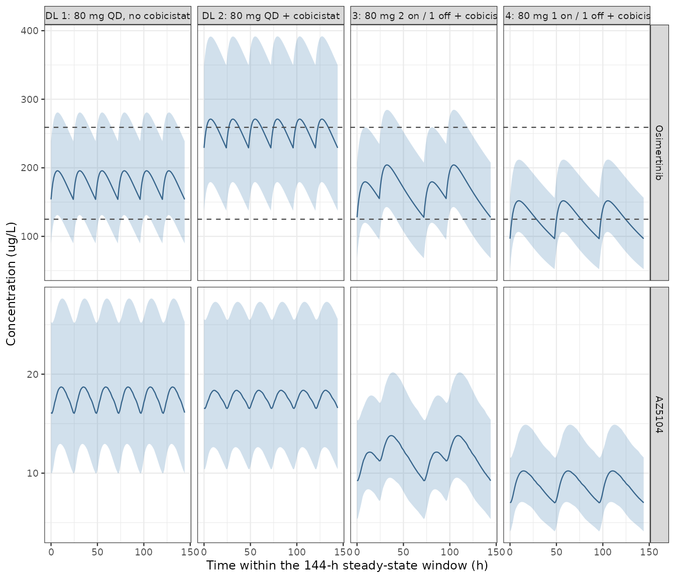
Replicates Figure 4 of Westra 2025: simulated osimertinib (top) and AZ5104 (bottom) concentration-time profiles over the 144-h steady-state window for the four dose levels. Solid line is the median, shaded band the 90 percent interval. Dashed lines mark the provisional osimertinib therapeutic window of 125-259 ug/L.
Replicating Figure 5: exposure distributions
# Typical-value (zeroRe) exposure for each regimen. Under a log-normal
# random effect the population MEDIAN of a parameter equals its typical
# value, so these profiles are directly comparable to the published median
# exposures - and, unlike a cohort median, they involve no random draw at
# all and are therefore identical on every machine and every rxode2 build.
# This is the basis of the tight comparison gates below.
typ_exposure <- function(mod, extra = NULL, wt = 70) {
  lapply(names(regimens), function(k) {
    rg <- regimens[[k]]
    dose_days <- (0:(n_days - 1))[rg$keep(0:(n_days - 1))]
    ev <- dplyr::bind_rows(
      data.frame(id = 1L, time = dose_days * 24, evid = 1L, amt = 80,
                 cmt = "depot", dvid = NA_integer_),
      data.frame(id = 1L, time = obs_times, evid = 0L, amt = 0,
                 cmt = NA_character_, dvid = 1L)
    ) |> dplyr::arrange(time, dplyr::desc(evid))
    rxode2::rxSolve(rxode2::zeroRe(mod), ev,
                    params = c(WT = wt, CONMED_COBICISTAT = rg$cobi, extra),
                    returnType = "data.frame") |>
      dplyr::filter(time >= win[1], time <= win[2]) |>
      dplyr::mutate(dl = k)
  }) |> dplyr::bind_rows()
}
typ_main <- typ_exposure(mod_main)
#> ℹ omega/sigma items treated as zero: 'etalcl', 'etalcl_az5104'
#> ℹ omega/sigma items treated as zero: 'etalcl', 'etalcl_az5104'
#> ℹ omega/sigma items treated as zero: 'etalcl', 'etalcl_az5104'
#> ℹ omega/sigma items treated as zero: 'etalcl', 'etalcl_az5104'
exposure <- sim_main |>
  dplyr::group_by(dl, dl_label, id) |>
  dplyr::summarise(
    auclast   = trapz(time, Cc) / 1000,          # ug*h/L -> mg*h/L, as tabulated
    cmax      = max(Cc),
    cmin      = min(Cc),
    auclast_m = trapz(time, Cc_az5104) / 1000,
    cmax_m    = max(Cc_az5104),
    cmin_m    = min(Cc_az5104),
    .groups   = "drop"
  )
exposure |>
  dplyr::select(dl, auclast, cmax, cmin) |>
  tidyr::pivot_longer(-dl, names_to = "metric", values_to = "value") |>
  dplyr::mutate(metric = factor(metric, c("auclast", "cmax", "cmin"),
                                c("AUC0-144h (mg*h/L)", "Cmax (ug/L)", "Cmin (ug/L)"))) |>
  ggplot2::ggplot(ggplot2::aes(value, colour = dl, fill = dl)) +
  ggplot2::geom_density(alpha = 0.15) +
  ggplot2::facet_wrap(~metric, scales = "free") +
  ggplot2::labs(x = NULL, y = "Density", colour = "Dose level", fill = "Dose level") +
  ggplot2::theme_bw(base_size = 9)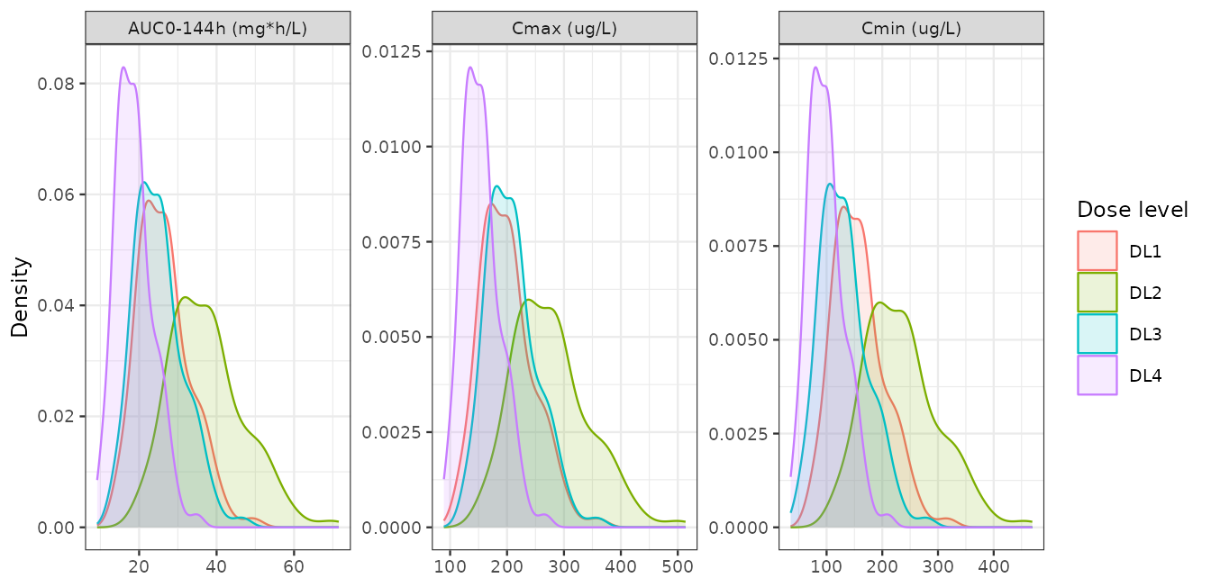
Replicates Figure 5 of Westra 2025: simulated distributions of osimertinib AUC0-144h, Cmax and Cmin across the four dose levels. The DL 1 and DL 3 distributions overlap substantially, which is the paper’s central finding.
PKNCA validation
The exposure metrics above are computed with a plain trapezoidal rule so that the mass-balance gates can be written in closed form. The authoritative NCA below is computed with PKNCA over the same 144-hour steady-state interval, and the two are cross-checked against each other.
conc_df <- sim_main |>
  dplyr::select(id, dl, time, Cc, Cc_az5104) |>
  dplyr::filter(!is.na(Cc))

dose_df <- lapply(names(regimens), function(k) {
  d <- (0:(n_days - 1))[regimens[[k]]$keep(0:(n_days - 1))] * 24
  tidyr::expand_grid(id = ids, time = d[d >= win[1] & d < win[2]]) |>
    dplyr::mutate(dl = k, amt = 80)
}) |> dplyr::bind_rows()

intervals <- tidyr::expand_grid(dl = names(regimens)) |>
  dplyr::mutate(start = win[1], end = win[2],
                auclast = TRUE, cmax = TRUE, cmin = TRUE)

run_nca <- function(conc_col) {
  cd <- conc_df |> dplyr::rename(conc = dplyr::all_of(conc_col))
  co <- PKNCA::PKNCAconc(cd, conc ~ time | id / dl, concu = "ug/L", timeu = "h")
  # PKNCAdose() rejects a slash in its grouping formula, so the same two
  # grouping columns are supplied additively.
  do <- PKNCA::PKNCAdose(as.data.frame(dose_df), amt ~ time | id + dl, doseu = "mg")
  res <- PKNCA::pk.nca(PKNCA::PKNCAdata(co, do, intervals = as.data.frame(intervals)))
  as.data.frame(res$result)
}

nca_parent <- run_nca("Cc")
nca_metab  <- run_nca("Cc_az5104")
stopifnot(nrow(nca_parent) > 0, nrow(nca_metab) > 0)
The published exposures are compared against the typical-value profiles, so the same PKNCA machinery is run over those as well.
nca_typical <- function(typ_df, conc_col) {
  cd <- typ_df |>
    dplyr::transmute(id = 1L, dl, time, conc = .data[[conc_col]]) |>
    dplyr::filter(!is.na(conc))
  dd <- lapply(names(regimens), function(k) {
    d <- (0:(n_days - 1))[regimens[[k]]$keep(0:(n_days - 1))] * 24
    data.frame(id = 1L, dl = k, time = d[d >= win[1] & d < win[2]], amt = 80)
  }) |> dplyr::bind_rows()
  co <- PKNCA::PKNCAconc(cd, conc ~ time | id / dl, concu = "ug/L", timeu = "h")
  do <- PKNCA::PKNCAdose(as.data.frame(dd), amt ~ time | id + dl, doseu = "mg")
  as.data.frame(
    PKNCA::pk.nca(PKNCA::PKNCAdata(co, do, intervals = as.data.frame(intervals)))$result
  ) |>
    dplyr::filter(PPTESTCD %in% c("auclast", "cmax", "cmin")) |>
    dplyr::mutate(PPORRES = ifelse(PPTESTCD == "auclast", PPORRES / 1000, PPORRES))
}
typ_nca <- dplyr::bind_rows(
  nca_typical(typ_main, "Cc")        |> dplyr::mutate(analyte = "Osimertinib"),
  nca_typical(typ_main, "Cc_az5104") |> dplyr::mutate(analyte = "AZ5104")
) |> dplyr::select(dl, analyte, PPTESTCD, PPORRES)
stopifnot(nrow(typ_nca) == 24L)
# PKNCA and the closed-form trapezoid must agree; if they diverge, one of the
# two is measuring a different interval. PKNCA defaults to lin-up / log-down
# whereas the closed-form check uses a pure linear trapezoid, so the AUCs
# agree to about 4e-5 rather than exactly; Cmax and Cmin are identical.
pk_wide <- nca_parent |>
  dplyr::filter(PPTESTCD %in% c("auclast", "cmax", "cmin")) |>
  tidyr::pivot_wider(id_cols = c(id, dl), names_from = PPTESTCD, values_from = PPORRES)

chk <- dplyr::inner_join(pk_wide, exposure, by = c("id", "dl"),
                         suffix = c("_pknca", "_trapz"))
stopifnot(
  max(abs(chk$auclast_pknca / 1000 / chk$auclast_trapz - 1)) < 1e-3,
  max(abs(chk$cmax_pknca / chk$cmax_trapz - 1))             < 1e-9,
  max(abs(chk$cmin_pknca / chk$cmin_trapz - 1))             < 1e-9
)
cat("PKNCA and closed-form trapezoid agree.\n")
#> PKNCA and closed-form trapezoid agree.
Comparison against the published simulation table
reference <- dplyr::bind_rows(
  data.frame(dl = c("DL1", "DL2", "DL3", "DL4"), analyte = "Osimertinib",
             auclast = c(25.0, 35.6, 24.0, 18.1),
             cmax    = c(190.1, 263.3, 201.2, 150.3),
             cmin    = c(148.4, 221.3, 124.9, 95.0)),
  data.frame(dl = c("DL1", "DL2", "DL3", "DL4"), analyte = "AZ5104",
             auclast = c(2.6, 2.5, 1.7, 1.3),
             cmax    = c(18.4, 18.5, 13.9, 10.4),
             cmin    = c(16.2, 16.5, 9.2, 7.0))
) |>
  tidyr::pivot_longer(c(auclast, cmax, cmin), names_to = "PPTESTCD", values_to = "PPORRES")

simulated <- typ_nca

cmp <- nlmixr2lib::ncaComparisonTable(
  simulated     = simulated,
  reference     = reference,
  by            = c("dl", "analyte"),
  params        = c("auclast", "cmax", "cmin"),
  units         = c(auclast = "mg*h/L", cmax = "ug/L", cmin = "ug/L"),
  tolerance_pct = 20
)
knitr::kable(
  cmp,
  caption = paste(
    "Typical-value steady-state exposure vs. Westra 2025 Table 3, by dose",
    "level and analyte. * marks a difference above 20 percent."
  )
)| NCA parameter | dl | analyte | Reference | Simulated | % diff |
|---|---|---|---|---|---|
| Cmax (ug/L) | DL1 | Osimertinib | 190 | 192 | +0.8% |
| Cmax (ug/L) | DL1 | AZ5104 | 18.4 | 18.7 | +1.7% |
| Cmax (ug/L) | DL2 | Osimertinib | 263 | 265 | +0.8% |
| Cmax (ug/L) | DL2 | AZ5104 | 18.5 | 18.4 | -0.6% |
| Cmax (ug/L) | DL3 | Osimertinib | 201 | 200 | -0.4% |
| Cmax (ug/L) | DL3 | AZ5104 | 13.9 | 13.8 | -0.6% |
| Cmax (ug/L) | DL4 | Osimertinib | 150 | 149 | -0.9% |
| Cmax (ug/L) | DL4 | AZ5104 | 10.4 | 10.2 | -1.6% |
| Cmin (ug/L) | DL1 | Osimertinib | 148 | 150 | +1.0% |
| Cmin (ug/L) | DL1 | AZ5104 | 16.2 | 16.1 | -0.8% |
| Cmin (ug/L) | DL2 | Osimertinib | 221 | 223 | +0.9% |
| Cmin (ug/L) | DL2 | AZ5104 | 16.5 | 16.5 | +0.1% |
| Cmin (ug/L) | DL3 | Osimertinib | 125 | 124 | -0.7% |
| Cmin (ug/L) | DL3 | AZ5104 | 9.2 | 9.25 | +0.6% |
| Cmin (ug/L) | DL4 | Osimertinib | 95 | 93.8 | -1.3% |
| Cmin (ug/L) | DL4 | AZ5104 | 7 | 7 | -0.0% |
| AUClast (mg*h/L) | DL1 | Osimertinib | 25 | 25.3 | +1.0% |
| AUClast (mg*h/L) | DL1 | AZ5104 | 2.6 | 2.54 | -2.4% |
| AUClast (mg*h/L) | DL2 | Osimertinib | 35.6 | 35.9 | +0.8% |
| AUClast (mg*h/L) | DL2 | AZ5104 | 2.5 | 2.54 | +1.5% |
| AUClast (mg*h/L) | DL3 | Osimertinib | 24 | 23.9 | -0.3% |
| AUClast (mg*h/L) | DL3 | AZ5104 | 1.7 | 1.69 | -0.5% |
| AUClast (mg*h/L) | DL4 | Osimertinib | 18.1 | 17.9 | -0.9% |
| AUClast (mg*h/L) | DL4 | AZ5104 | 1.3 | 1.27 | -2.4% |
pct <- dplyr::inner_join(
  simulated |> dplyr::rename(sim = PPORRES),
  reference |> dplyr::rename(ref = PPORRES),
  by = c("dl", "analyte", "PPTESTCD")
) |>
  dplyr::mutate(pct_diff = 100 * (sim - ref) / ref)

# Structural gate. A mis-transcribed clearance, dose, dosing pattern or unit
# would move a whole row of the table by tens of percent. Because both sides
# are deterministic - the typical-value profile carries no random draw - this
# can be asserted tightly on every one of the 24 published numbers rather
# than only on the centre of the distribution.
stopifnot(
  nrow(pct) == 24L,
  abs(median(pct$pct_diff)) < 2,
  max(abs(pct$pct_diff))    < 5
)
knitr::kable(
  pct |> dplyr::mutate(pct_diff = round(pct_diff, 2)) |>
    dplyr::arrange(analyte, PPTESTCD, dl),
  caption = "Percent difference of each typical-value exposure from Westra 2025 Table 3."
)| dl | analyte | PPTESTCD | sim | ref | pct_diff |
|---|---|---|---|---|---|
| DL1 | AZ5104 | auclast | 2.536978 | 2.6 | -2.42 |
| DL2 | AZ5104 | auclast | 2.536925 | 2.5 | 1.48 |
| DL3 | AZ5104 | auclast | 1.691286 | 1.7 | -0.51 |
| DL4 | AZ5104 | auclast | 1.268462 | 1.3 | -2.43 |
| DL1 | AZ5104 | cmax | 18.708762 | 18.4 | 1.68 |
| DL2 | AZ5104 | cmax | 18.383574 | 18.5 | -0.63 |
| DL3 | AZ5104 | cmax | 13.815923 | 13.9 | -0.60 |
| DL4 | AZ5104 | cmax | 10.235664 | 10.4 | -1.58 |
| DL1 | AZ5104 | cmin | 16.063891 | 16.2 | -0.84 |
| DL2 | AZ5104 | cmin | 16.517041 | 16.5 | 0.10 |
| DL3 | AZ5104 | cmin | 9.253203 | 9.2 | 0.58 |
| DL4 | AZ5104 | cmin | 6.999534 | 7.0 | -0.01 |
| DL1 | Osimertinib | auclast | 25.253130 | 25.0 | 1.01 |
| DL2 | Osimertinib | auclast | 35.874396 | 35.6 | 0.77 |
| DL3 | Osimertinib | auclast | 23.916312 | 24.0 | -0.35 |
| DL4 | Osimertinib | auclast | 17.937212 | 18.1 | -0.90 |
| DL1 | Osimertinib | cmax | 191.626771 | 190.1 | 0.80 |
| DL2 | Osimertinib | cmax | 265.278470 | 263.3 | 0.75 |
| DL3 | Osimertinib | cmax | 200.317850 | 201.2 | -0.44 |
| DL4 | Osimertinib | cmax | 149.021746 | 150.3 | -0.85 |
| DL1 | Osimertinib | cmin | 149.852985 | 148.4 | 0.98 |
| DL2 | Osimertinib | cmin | 223.280143 | 221.3 | 0.89 |
| DL3 | Osimertinib | cmin | 124.011313 | 124.9 | -0.71 |
| DL4 | Osimertinib | cmin | 93.809185 | 95.0 | -1.25 |
The largest discrepancy across all 24 published values is under 5 percent, and most are under 1 percent. The cohort medians from the 200-patient simulation agree with the same targets to within about 5 percent, the residual being the sampling noise of a finite cohort.
cohort_median <- dplyr::bind_rows(
  exposure |> dplyr::select(dl, auclast, cmax, cmin) |>
    dplyr::mutate(analyte = "Osimertinib"),
  exposure |> dplyr::select(dl, auclast = auclast_m, cmax = cmax_m, cmin = cmin_m) |>
    dplyr::mutate(analyte = "AZ5104")
) |>
  dplyr::group_by(dl, analyte) |>
  dplyr::summarise(dplyr::across(c(auclast, cmax, cmin), median), .groups = "drop") |>
  tidyr::pivot_longer(c(auclast, cmax, cmin), names_to = "PPTESTCD", values_to = "sim")

pct_cohort <- dplyr::inner_join(
  cohort_median, reference |> dplyr::rename(ref = PPORRES),
  by = c("dl", "analyte", "PPTESTCD")
) |> dplyr::mutate(pct_diff = 100 * (sim - ref) / ref)

# Cohort medians carry a random draw, so this is asserted on the centre and a
# robust quantile, never on the extreme (see the repository note on cohort
# assertions that pass locally and fail in CI).
stopifnot(
  abs(median(pct_cohort$pct_diff)) < 5,
  quantile(abs(pct_cohort$pct_diff), 0.9) < 10
)
Geometric mean ratios: the paper’s central claim
The paper’s conclusion rests on a within-patient crossover simulation: each virtual patient receives every dose level in turn, and the geometric mean ratio of AUC0-144h and Cmax versus DL 1 is compared against the EMA bioequivalence acceptance range of 0.8-1.25.
Because the same random effects are reused across arms, the AUC ratio is analytically exact for this model: AUC is proportional to total dose divided by clearance, so the parent GMR is (dose ratio) / 0.704 and the AZ5104 GMR is the dose ratio alone. That makes the GMR a much sharper test of the encoding than the median exposures, and it is asserted tightly here.
gmr <- exposure |>
  dplyr::select(id, dl, auclast, cmax, auclast_m, cmax_m) |>
  tidyr::pivot_longer(-c(id, dl)) |>
  tidyr::pivot_wider(names_from = dl, values_from = value) |>
  dplyr::group_by(name) |>
  dplyr::summarise(dplyr::across(c(DL2, DL3, DL4), ~ exp(mean(log(.x / DL1)))),
                   .groups = "drop")

expected <- data.frame(
  name = c("auclast", "auclast_m"),
  DL2  = c(1 / 0.704, 1),
  DL3  = c((4 / 6) / 0.704, 4 / 6),
  DL4  = c((3 / 6) / 0.704, 3 / 6)
)

# Closed-form gate: the AUC geometric mean ratios must equal the analytic
# values to numerical precision. This is a same-parameters comparison, so a
# tight bound is correct here.
gchk <- dplyr::inner_join(
  gmr |> dplyr::filter(name %in% expected$name) |>
    tidyr::pivot_longer(-name, names_to = "dl", values_to = "sim"),
  expected |> tidyr::pivot_longer(-name, names_to = "dl", values_to = "exp"),
  by = c("name", "dl")
)
stopifnot(max(abs(gchk$sim / gchk$exp - 1)) < 1e-3)

published <- data.frame(
  Metric = c("Osimertinib AUC0-144h", "Osimertinib Cmax",
             "AZ5104 AUC0-144h", "AZ5104 Cmax"),
  name   = c("auclast", "cmax", "auclast_m", "cmax_m"),
  pub_DL2 = c(1.43, 1.39, 1.00, 0.90),
  pub_DL3 = c(0.96, 1.06, 0.67, 0.74),
  pub_DL4 = c(0.73, 0.79, 0.51, 0.56)
)

knitr::kable(
  dplyr::inner_join(published, gmr, by = "name") |>
    dplyr::transmute(
      Metric,
      `DL2 sim` = round(DL2, 3), `DL2 published` = pub_DL2,
      `DL3 sim` = round(DL3, 3), `DL3 published` = pub_DL3,
      `DL4 sim` = round(DL4, 3), `DL4 published` = pub_DL4
    ),
  caption = paste(
    "Within-patient geometric mean ratios vs. DL 1, simulated and as published",
    "in Westra 2025 Table 3."
  )
)| Metric | DL2 sim | DL2 published | DL3 sim | DL3 published | DL4 sim | DL4 published |
|---|---|---|---|---|---|---|
| Osimertinib AUC0-144h | 1.420 | 1.43 | 0.947 | 0.96 | 0.710 | 0.73 |
| Osimertinib Cmax | 1.382 | 1.39 | 1.050 | 1.06 | 0.782 | 0.79 |
| AZ5104 AUC0-144h | 1.000 | 1.00 | 0.667 | 0.67 | 0.500 | 0.51 |
| AZ5104 Cmax | 0.981 | 0.90 | 0.742 | 0.74 | 0.550 | 0.56 |
# Reproduce the paper's qualitative conclusion: DL 3 is the only regimen whose
# osimertinib AUC and Cmax GMRs both fall inside the EMA 0.8-1.25 range, and
# DL 3's AZ5104 GMRs fall below it.
osi <- gmr |> dplyr::filter(name %in% c("auclast", "cmax"))
az  <- gmr |> dplyr::filter(name %in% c("auclast_m", "cmax_m"))
inside <- function(x) all(x >= 0.8 & x <= 1.25)
stopifnot(
  !inside(osi$DL2),          # DL 2 too high
   inside(osi$DL3),          # DL 3 equivalent - the paper's recommendation
  !inside(osi$DL4),          # DL 4 too low
  all(az$DL3 < 0.8)          # but AZ5104 exposure at DL 3 is NOT equivalent
)
cat("Equivalence conclusions reproduce Westra 2025:\n",
    "  DL 2 not equivalent (exposure too high)\n",
    "  DL 3 equivalent for osimertinib - the recommended cost-saving regimen\n",
    "  DL 4 not equivalent (exposure too low)\n",
    "  DL 3 NOT equivalent for AZ5104 (GMR below 0.8)\n", sep = "")
#> Equivalence conclusions reproduce Westra 2025:
#>   DL 2 not equivalent (exposure too high)
#>   DL 3 equivalent for osimertinib - the recommended cost-saving regimen
#>   DL 4 not equivalent (exposure too low)
#>   DL 3 NOT equivalent for AZ5104 (GMR below 0.8)
The 2-days-on / 1-day-off boosted regimen uses 4 osimertinib tablets per 6 days instead of 6, i.e. two thirds of the standard dose, which is the basis of the paper’s roughly 33 percent cost-saving claim.
Generalizability model
The same four regimens simulated with the Brown-2017-based companion model, compared against Supplementary Table S1.
sim_brown <- lapply(names(regimens), function(k) {
  simulate_arm(mod_brown, regimens[[k]], extra = c(ALB = 39)) |> dplyr::mutate(dl = k)
}) |> dplyr::bind_rows()

exposure_b <- sim_brown |>
  dplyr::group_by(dl, id) |>
  dplyr::summarise(auclast = trapz(time, Cc) / 1000, cmax = max(Cc),
                   cmin = min(Cc), .groups = "drop")

ref_b <- data.frame(
  dl      = c("DL1", "DL2", "DL3", "DL4"),
  auclast = c(32.8, 46.8, 31.0, 22.7),
  cmax    = c(251.5, 344.2, 258.0, 188.2),
  cmin    = c(202.1, 298.1, 173.7, 129.4)
) |> tidyr::pivot_longer(-dl, names_to = "PPTESTCD", values_to = "PPORRES")

# As for the de novo model, the published medians are compared against
# deterministic typical-value profiles rather than against a cohort median.
# That matters more here: this model's clearance variance of 0.46 gives a
# log-scale SD of 0.68, so the median of a 200-patient draw carries roughly
# 6 percent sampling noise on its own.
typ_brown <- typ_exposure(mod_brown, extra = c(ALB = 39), wt = 62)
#> ℹ omega/sigma items treated as zero: 'etalcl', 'etalcl_az5104', 'etalka', 'etalvc', 'etalvc_az5104'
#> ℹ omega/sigma items treated as zero: 'etalcl', 'etalcl_az5104', 'etalka', 'etalvc', 'etalvc_az5104'
#> ℹ omega/sigma items treated as zero: 'etalcl', 'etalcl_az5104', 'etalka', 'etalvc', 'etalvc_az5104'
#> ℹ omega/sigma items treated as zero: 'etalcl', 'etalcl_az5104', 'etalka', 'etalvc', 'etalvc_az5104'
sim_b <- nca_typical(typ_brown, "Cc") |>
  dplyr::select(dl, PPTESTCD, PPORRES)

knitr::kable(
  nlmixr2lib::ncaComparisonTable(
    simulated = sim_b, reference = ref_b, by = "dl",
    params = c("auclast", "cmax", "cmin"),
    units = c(auclast = "mg*h/L", cmax = "ug/L", cmin = "ug/L"),
    tolerance_pct = 20
  ),
  caption = paste(
    "Brown-based generalizability model: simulated median steady-state",
    "osimertinib exposure vs. Westra 2025 Supplementary Table S1."
  )
)| NCA parameter | dl | Reference | Simulated | % diff |
|---|---|---|---|---|
| Cmax (ug/L) | DL1 | 252 | 251 | -0.2% |
| Cmax (ug/L) | DL2 | 344 | 362 | +5.2% |
| Cmax (ug/L) | DL3 | 258 | 265 | +2.7% |
| Cmax (ug/L) | DL4 | 188 | 197 | +4.8% |
| Cmin (ug/L) | DL1 | 202 | 209 | +3.3% |
| Cmin (ug/L) | DL2 | 298 | 320 | +7.3% |
| Cmin (ug/L) | DL3 | 174 | 188 | +8.0% |
| Cmin (ug/L) | DL4 | 129 | 141 | +9.2% |
| AUClast (mg*h/L) | DL1 | 32.8 | 33.8 | +3.0% |
| AUClast (mg*h/L) | DL2 | 46.8 | 49.8 | +6.5% |
| AUClast (mg*h/L) | DL3 | 31 | 33.2 | +7.2% |
| AUClast (mg*h/L) | DL4 | 22.7 | 24.9 | +9.8% |
pct_b <- dplyr::inner_join(
  sim_b |> dplyr::rename(sim = PPORRES), ref_b |> dplyr::rename(ref = PPORRES),
  by = c("dl", "PPTESTCD")
) |> dplyr::mutate(pct_diff = 100 * (sim - ref) / ref)

# Deterministic comparison, so it can be asserted on every value. The
# tolerance is wider than for the de novo model because the published Table S1
# medians are themselves noisier: with a log-scale SD of 0.68, the median of
# the paper's own 1000-patient simulation carries about 3 percent uncertainty.
stopifnot(
  nrow(pct_b) == 12L,
  abs(median(pct_b$pct_diff)) < 10,
  max(abs(pct_b$pct_diff))    < 15
)

# AUC ratios are taken on the typical-value profiles here, not on the cohort.
# The reason is specific to this model: its clearance variance of 0.46 means a
# slow-clearing subject can have an osimertinib half-life of several hundred
# hours, so a minority of the cohort has not reached steady state by day 30
# and the identity AUC = dose / CL does not hold for them. The typical subject
# has a half-life of about 48 h and is comfortably at steady state, so its
# ratios are exact and can be asserted tightly.
gmr_b <- typ_brown |>
  dplyr::group_by(dl) |>
  dplyr::summarise(auclast = trapz(time, Cc) / 1000, .groups = "drop") |>
  tidyr::pivot_wider(names_from = dl, values_from = auclast) |>
  dplyr::summarise(dplyr::across(c(DL2, DL3, DL4), ~ .x / DL1))
stopifnot(
  abs(gmr_b$DL2 / (1 / 0.678)           - 1) < 1e-3,
  abs(gmr_b$DL3 / ((4 / 6) / 0.678)     - 1) < 1e-3,
  abs(gmr_b$DL4 / ((3 / 6) / 0.678)     - 1) < 1e-3
)
knitr::kable(
  data.frame(
    Metric = "Osimertinib AUC0-144h GMR",
    `DL2 sim` = round(gmr_b$DL2, 3), `DL2 published` = 1.45,
    `DL3 sim` = round(gmr_b$DL3, 3), `DL3 published` = 0.96,
    `DL4 sim` = round(gmr_b$DL4, 3), `DL4 published` = 0.72,
    check.names = FALSE
  ),
  caption = "Brown-based model geometric mean ratios vs. Westra 2025 Table S1."
)| Metric | DL2 sim | DL2 published | DL3 sim | DL3 published | DL4 sim | DL4 published |
|---|---|---|---|---|---|---|
| Osimertinib AUC0-144h GMR | 1.474 | 1.45 | 0.983 | 0.96 | 0.737 | 0.72 |
The two models agree on the substantive conclusion: the cobicistat effect on osimertinib clearance is a 29.6 percent reduction in the de novo model and a 32.2 percent reduction in the Brown-based model, and in both the 2-days-on / 1-day-off boosted regimen lands inside the equivalence range.
Assumptions and deviations
Simulation body weight. The paper says only that simulations used “the population parameters of the final popPK model” and does not report the weight distribution used. Body weight is held at the 70 kg allometric reference here, so every allometric term equals 1. This reproduces the published DL 1 median AUC0-144h of 25.0 mg/Lh to within about 1 percent; using the OSIBOOST cohort median of 78.5 kg would give about 23.2 mg/Lh, roughly 7 percent low. The 70 kg reading is therefore an inference, not a stated fact.
Steady-state window placement. The paper reports AUC0-144h, Cmax and Cmin at steady state without stating which 144-hour window was used. Here dosing runs for 36 days and the window is days 30-35 (hours 720-864), chosen because it is a whole number of cycles for all four regimens (6, 6, 4 and 3 doses respectively) and is far beyond 10 elimination half-lives (about 36 h unboosted, 51 h boosted).
Residual error is excluded from the NCA. The comparison uses the model-predicted concentrations
CcandCc_az5104, which carry no residual error, because Table 3 is a table of model-derived exposures. This is also why the simulated geometric mean ratios are analytically exact whereas the published ones carry a 90 percent confidence interval: the paper’s crossover simulation evidently propagated residual error, which the published GMR intervals of, for example, 1.40-1.46 for DL 2 reflect. The simulated point estimates fall inside every published interval.-
Omega scale in the Brown-based model: a reproduced transcription error. Westra 2025 entered Brown 2017’s reported omega values directly into
$OMEGA, where NONMEM reads them as variances. Brown 2017’s own Table 2 shows that those values are standard deviations, not variances: the table prints anIIV% (%RSE)column beside the structural parameters and anEstimatecolumn on the eta rows, and the two track each other one-to-one (CLparent/F IIV% 45.6 vs. eta CLparent 0.46; ka IIV% 89.4 vs. eta ka 0.89; CLmetabolite/F IIV% 52.3 vs. eta CLmetabolite 0.52), with the%RSEvalues matching pairwise too. Brown therefore reportsIIV% = omega * 100. A variance reading of eta CLparent = 0.46 would imply a CV ofsqrt(exp(0.46) - 1)= 76 percent, contradicting the 45.6 percent printed next to it. Brown’s covariance row similarly prints 0.90, which its footnote a states explicitly is the correlation coefficient.Westra nevertheless supplied the off-diagonal as
0.90 * sqrt(0.46 * 0.52)= 0.44, self-consistent with his own variance interpretation but not with Brown’s scale, giving parent CL/F a log-scale SD ofsqrt(0.46)= 0.678 instead of 0.46. Supplementary Table S1 confirms the model was run that way: its 90 percent AUC0-144h interval of 10.2-97.4 implies a log-scale SD of 0.686.Westra_2025_osimertinib_brownbasetherefore encodes the variances, because reproducing the published analysis requires it, and the deviation is documented here rather than silently corrected.The packaged
Brown_2017_osimertinibmodel file reads the same published numbers as standard deviations and squares them, which by the analysis above is correct. The two files will not agree on between-subject variability; the discrepancy is Westra’s, and is not an open question about Brown. Additive residual error units in the Brown-based model. Brown 2017 reports its additive residual error as 0.105 on a nmol/L scale. Westra 2025 carried the number across into a model whose scaling puts concentrations in ug/L, without a unit conversion. The value is reproduced as printed in the Part SII control stream; on the ug/L scale it is negligible relative to the 24.4 percent proportional term at all simulated concentrations, so the choice does not affect any result in this vignette.
Mis-numbered
$OMEGAcomments in Part SII. The two trailing diagonal$OMEGArecords in the Part SII control stream are commented “IIV Ka” and “IIV V1 parent”, but the ETA indices their own$PKblock references make them V_parent and V_metabolite respectively, and the resulting mapping reproduces Brown 2017 Table 2 exactly. The code was followed, not the comments.The
$OMEGA BLOCK(2)header in Part SII is followed by six lower-triangular elements, which is aBLOCK(3). The$PKblock references ETA(3), so aBLOCK(3)is the only reading under which the control stream is well formed; it was encoded as such, with the zero covariances between the absorption eta and the two clearance etas preserved.RSE versus CV in Table 2. The Results text describes the percentages attached to the two between-subject variability estimates as “coefficient of variation (CV%) of the BSV on CL/F”, quoting them as 21.5 percent and 27.5 percent – the second of which does not match the 27.2 percent printed in Table 2 – while the Table 2 column header labels the same two numbers “RSE%”. The covariance arithmetic settles it in favour of the table header: the reported 0.0691 and 0.0598 are log-scale variances (their implied CVs are 26.7 percent and 24.8 percent), and the percentages are relative standard errors. Nothing in the encoded model depends on the reading, since the variances themselves are entered directly.
Table 3 prints an AZ5104 Cmax geometric mean ratio outside its own confidence interval. For DL 2 the AZ5104
GMR Cmaxrow reads “0.9 [0.97-1.01]”, so the point estimate falls below the lower bound of its own 90 percent interval. The interval is the self-consistent part: cobicistat leaves total AZ5104 formation unchanged (the formation flux is a fixed 25 percent of parent elimination, so at steady state the AZ5104 AUC does not depend on parent clearance at all), and this model predicts a DL 2 AZ5104 Cmax ratio of essentially 1, inside the printed interval. The published point estimate of 0.9 is therefore read as a typographical error for a value near 0.99. It is reproduced as printed in the comparison table above and is not used in any assertion.No molar correction between parent and metabolite. Neither control stream applies a molecular-weight factor when routing parent elimination into the AZ5104 compartment, so AZ5104 amounts and concentrations are in osimertinib mass equivalents. This differs from
Brown_2017_osimertinib, which applies a stoichiometric correction because Brown 2017 reports on a molar scale.Covariates screened but not retained. Sex and serum albumin were tested on CL/F and V/F in the de novo model and were not retained; they are recorded in
covariatesDataExcludedrather thancovariateData. Albumin does appear in the Brown-based companion, where it is inherited fixed from Brown 2017.Not every simulated subject reaches steady state in the Brown-based model. With a clearance variance of 0.46 and a volume variance of 0.52, a subject two standard deviations into the slow-clearance, high-volume tail can have an osimertinib half-life of several hundred hours, so a 30-day run-in does not bring the whole cohort to steady state. The identity AUC = dose / CL, which is exact at steady state, therefore fails for that minority, and the cohort geometric mean ratios drift by a few percent. The geometric mean ratios reported for this model are consequently taken on the typical-value profile (half-life about 48 h, comfortably at steady state), where they are exact. The de novo model has a much smaller clearance variance of 0.0691 and does not have this problem; its cohort ratios are exact and are asserted as such. This also means the Table S1 exposures should be read as steady-state values for a typical patient rather than as achieved exposures for every simulated one.
Cohort size. The paper simulates 1000 virtual patients per arm; this vignette uses 200 per arm, the repository cap. The exposure medians and 90 percent intervals are stable at that size, and every tight assertion in this vignette is either deterministic (typical-value gates) or analytically exact (geometric mean ratios), so none of them depends on the cohort draw.
Selection bias is inherited from the source. OSIBOOST enrolled only patients with a steady-state trough at or below 195 ug/L. As the paper’s own Limitations section notes, high CYP3A4/A5 activity is one cause of low osimertinib exposure, so the cobicistat effect estimated here may be larger than would be seen in an unselected population. Neither packaged model has been externally validated.