Piperaquine malaria chemoprevention in young children (Wallender 2021)
Source:vignettes/articles/Wallender_2021_piperaquine.Rmd
Wallender_2021_piperaquine.RmdModel and source
Wallender 2021 reports three models built on one randomised trial of intermittent preventive treatment (IPT) with dihydroartemisinin-piperaquine (DP) in Ugandan children. They were fitted sequentially rather than jointly, so each is packaged as its own model file; all three point at this article.
mods <- c(
  "Wallender_2021_piperaquine",
  "Wallender_2021_piperaquine_malaria",
  "Wallender_2021_piperaquine_qtc"
)
ui <- lapply(mods, function(n) rxode2::rxode(readModelDb(n)))
#> Warning: some etas defaulted to non-mu referenced, possible parsing error: etaiov_fdepot_1, etaiov_fdepot_2, etaiov_fdepot_3, etaiov_fdepot_4, etaiov_fdepot_5, etaiov_fdepot_6, etaiov_fdepot_7, etaiov_fdepot_8, etaiov_fdepot_9, etaiov_fdepot_10, etaiov_fdepot_11, etaiov_fdepot_12, etaiov_fdepot_13, etaiov_fdepot_14, etaiov_fdepot_15, etaiov_fdepot_16, etaiov_fdepot_17, etaiov_fdepot_18, etaiov_fdepot_19, etaiov_fdepot_20, etaiov_fdepot_21, etaiov_fdepot_22, etaiov_fdepot_23, etaiov_fdepot_24, etaiov_fdepot_25
#> as a work-around try putting the mu-referenced expression on a simple line
#> Warning: some etas defaulted to non-mu referenced, possible parsing error: etaiov_fdepot_1, etaiov_fdepot_2, etaiov_fdepot_3, etaiov_fdepot_4, etaiov_fdepot_5, etaiov_fdepot_6, etaiov_fdepot_7, etaiov_fdepot_8, etaiov_fdepot_9, etaiov_fdepot_10, etaiov_fdepot_11, etaiov_fdepot_12, etaiov_fdepot_13, etaiov_fdepot_14, etaiov_fdepot_15, etaiov_fdepot_16, etaiov_fdepot_17, etaiov_fdepot_18, etaiov_fdepot_19, etaiov_fdepot_20, etaiov_fdepot_21, etaiov_fdepot_22, etaiov_fdepot_23, etaiov_fdepot_24, etaiov_fdepot_25
#> as a work-around try putting the mu-referenced expression on a simple line
#> Warning: some etas defaulted to non-mu referenced, possible parsing error: etaiov_fdepot_1, etaiov_fdepot_2, etaiov_fdepot_3, etaiov_fdepot_4, etaiov_fdepot_5, etaiov_fdepot_6, etaiov_fdepot_7, etaiov_fdepot_8, etaiov_fdepot_9, etaiov_fdepot_10, etaiov_fdepot_11, etaiov_fdepot_12, etaiov_fdepot_13, etaiov_fdepot_14, etaiov_fdepot_15, etaiov_fdepot_16, etaiov_fdepot_17, etaiov_fdepot_18, etaiov_fdepot_19, etaiov_fdepot_20, etaiov_fdepot_21, etaiov_fdepot_22, etaiov_fdepot_23, etaiov_fdepot_24, etaiov_fdepot_25
#> as a work-around try putting the mu-referenced expression on a simple line
names(ui) <- mods

# rxSolve returns the occasion column OCC twice for these models - once as the
# model-visible covariate that the IOV indicators compare against, and once as
# the input column passed through - and dplyr refuses to work on a data frame
# with duplicate names. Both copies hold the same values, so the second is
# dropped. Applied to every solve below.
as_sim_df <- function(x) {
  d <- as.data.frame(x)
  d[, !duplicated(names(d)), drop = FALSE]
}- Citation: Wallender E, Ali AM, Hughes E, Kakuru A, Jagannathan P, Muhindo MK, Opira B, Whalen M, Huang L, Duvalsaint M, Legac J, Kamya MR, Dorsey G, Aweeka F, Rosenthal PJ, Savic RM. Identifying an optimal dihydroartemisinin-piperaquine dosing regimen for malaria prevention in young Ugandan children. Nat Commun. 2021;12(1):6714. doi:10.1038/s41467-021-27051-8. PMC8602248. Open Access under CC BY 4.0. Final parameter estimates are in Table 2; the structural equations are Eq. 1 (clearance) and Eq. 2 (bioavailability) with the capillary-to-venous conversion in Table 2 footnote c. The Peer Review File (41467_2021_27051_MOESM2_ESM.pdf) carries a SUPERSEDED earlier revision of Table 2 in which clearance is 435 L/d with a power function of age; those values must not be used. Sister model files from the same paper: modellib(‘Wallender_2021_piperaquine_malaria’) and modellib(‘Wallender_2021_piperaquine_qtc’).
- Article: https://doi.org/10.1038/s41467-021-27051-8
- Source Data (Figures 5B, 6A, 6B, 6C): https://static-content.springer.com/esm/art%3A10.1038%2Fs41467-021-27051-8/MediaObjects/41467_2021_27051_MOESM4_ESM.xlsx
| Model file | What it describes | Endpoint |
|---|---|---|
Wallender_2021_piperaquine |
Population PK of piperaquine; three-compartment disposition, two transit absorption compartments, joint venous plus capillary sampling | Cc |
Wallender_2021_piperaquine_malaria |
Repeated time to incident malaria; exponential baseline hazard, transmission-period multiplier, sigmoidal drug protection | sur |
Wallender_2021_piperaquine_qtc |
Linear concentration-QTcB relationship on the intensive-PK substudy | QTcB |
A fourth analysis in the paper, a logistic regression of pfmdr1 / pfcrt mutant-parasite detection on piperaquine concentration, reports no parameter values at all - only that “time-varying PPQ concentration was not significantly associated with the probability of detecting a mutant parasite”. There is nothing numeric to encode, so no model file exists for it. This is a reporting gap in the source, not a narrowing of scope.
Population
pop <- ui[[1]]$population
str(pop, max.level = 1, give.attr = FALSE)
#> List of 11
#>  $ species       : chr "human"
#>  $ n_subjects    : int 280
#>  $ n_studies     : int 1
#>  $ age_range     : chr "2 to 36 months (dosed from 8 to 104 weeks of age; PK sampled from 12 to 104 weeks)"
#>  $ weight_median : chr "8.6 kg (study median, used as the allometric reference)"
#>  $ sex_female_pct: num 48.9
#>  $ disease_state : chr "Healthy Ugandan infants and toddlers born to mothers enrolled in a trial of intermittent preventive treatment i"| __truncated__
#>  $ dose_range    : chr "Weight-band dosed dihydroartemisinin-piperaquine once daily for three consecutive days per course: <6 kg 10/80 "| __truncated__
#>  $ regions       : chr "Tororo District, Uganda"
#>  $ n_observations: int 4573
#>  $ notes         : chr "Randomised controlled trial NCT02163447; participant characteristics in Table 1. 4573 PPQ concentrations, of wh"| __truncated__
280 Ugandan children (NCT02163447) born in Tororo District were randomised before birth to receive a three-day DP course every 12 weeks (n = 184) or every 4 weeks (n = 96) from 8 to 104 weeks of age, and were followed to 36 months. Doses were assigned by weight band from the manufacturer’s package insert (Supplementary Table 1). Baseline characteristics are in Table 1: median birth weight 3000 g and 2965 g in the two arms, median gestational age 39.9 and 39.0 weeks, 11.4% and 14.6% of low birth weight, and a median weight-for-age z-score at 8 weeks of -0.22 and -0.31. The study-median body weight of 8.6 kg is the allometric reference for every disposition parameter.
The PK model was fitted to 4573 piperaquine concentrations, of which 578 (12.6%) were below the 0.5 ng/mL limit of quantification and were handled by the M6 (BLQ/2) method. All children contributed sparse samples; 32 children also contributed intensive profiles at 32 and 104 weeks of age, and those 32 contributed the paired electrocardiograms behind the QTc model. The hazard model was fitted to 326 incident-malaria episodes.
Source trace
Every value below is transcribed from the source; none is derived or
assumed. Per-parameter provenance is also recorded as an in-file comment
beside each ini() entry.
| Equation / parameter | Value | Source location |
|---|---|---|
lcl (CL/F, fully mature) |
867 L/day | Table 2, Clearance |
ltm50_cl |
96 weeks | Table 2, theta Post menstrual age EC50 |
lvc |
592 L | Table 2, Volume of central compartment |
lq |
511 L/day | Table 2, Intercompartmental clearance 1 |
lvp |
7240 L | Table 2, Volume of peripheral compartment 1 |
lq2 |
671 L/day | Table 2, Intercompartmental clearance 2 |
lvp2 |
1060 L | Table 2, Volume of peripheral compartment 2 |
lmtt |
0.045 day | Table 2, Absorption transit time |
e_wt_cl, e_wt_vc
|
0.75, 1 | Methods, “Population PK model” (a priori, not estimated) |
lfdepot |
1 | Table 2, Relative bioavailability (F); pre-specified anchor |
e_waz_fdepot |
0.113 | Table 2, theta Weight for age z-score |
e_selfadmin_fdepot |
0.397 | Table 2, theta Self-administered DP |
e_sample_capillary_cc |
0.922 | Table 2 footnote c |
propSd |
0.446 | Table 2, Proportional error |
| IIV on CL, Vc, MTT | 27.1%, 32.8%, 43.2% | Table 2, interindividual-variability column |
| BOV on F | 66.9% | Table 2, theta Between occasion variability |
CL = theta_CL * (WT/8.6)^0.75 * PMA/(PMA + theta_EC50) * exp(eta) |
n/a | Equation 1 |
F = theta_F * (1 + theta_WAZ * (WAZ + 0.5)) * theta_SelfAdmin * exp(BOV) |
n/a | Equation 2 and Table 2 footnote d |
lhaz_base |
0.402 / 1000 per day | Table 2, Baseline hazard/1000 |
| transmission multipliers 2015 / 2016 / 2017 | 1.29 / 5.20 / 7.83 | Table 2, theta Transmission period |
lec50 (malaria) |
6.00 ng/mL | Table 2, theta PPQ EC50 |
lhill (malaria) |
3.13 | Table 2, theta PPQ gamma |
| IIV on baseline hazard | 69.6% | Table 2, interindividual-variability column |
hazard = h0 * transmission * (1 - C^g/(EC50^g + C^g)) * exp(eta) |
n/a | Equation 3 |
le0_qtc |
410 msec | Supplementary Table 2, Pre-drug QTcB |
e_ppq_qtc |
0.0463 msec per ng/mL | Supplementary Table 2, theta Slope |
| IIV on pre-drug QTcB | 1.4% | Supplementary Table 2 |
Interindividual variability is tabulated as %CV and converted to the
log-normal variance with omega^2 = log(CV^2 + 1).
Two printed-source readings had to be adjudicated; both are recorded in Assumptions and deviations below and in the model files.
Virtual cohort
The trial data are not public, so the cohorts below are virtual. Two covariate distributions are anchored on published values rather than assumed: body weight follows a smooth curve pinned to the median birth weight of 3000 g at age 0 and to the study-median 8.6 kg at the median postnatal age of 57 weeks, and the weight-for-age z-score is drawn around the cohort median of -0.5 that Equation 2 centres on, with a spread matching the 2.5-97.5 percentile range in Table 1.
# rxSetSeed() fixes rxode2's stream per solver thread, not across thread counts,
# so a CI runner with a different core count draws a different cohort. Every
# assertion below is written to hold for any cohort this model can produce.
set.seed(20211122)
rxode2::rxSetSeed(20211122)

# Body weight (kg) as a function of postnatal age in weeks. Pinned at both ends
# to published values: 3.0 kg at birth (Table 1 median birth weight 3000 g) and
# 8.6 kg at 57 weeks (Methods; the allometric reference and the cohort median
# postnatal age). Sits about 0.5 z-score below the WHO median, consistent with
# the cohort's own median WAZ of -0.5.
wt_for_age <- function(week) 3.0 + 5.6 * (pmax(week, 0) / 57)^0.55

# Weight-band daily piperaquine dose (mg), clinical trial protocol
# (Supplementary Table 1).
dose_protocol <- function(wt) {
  ifelse(wt < 6, 80, ifelse(wt < 11, 160, ifelse(wt < 15, 240, 320)))
}
# World Health Organization 2015 treatment guideline bands.
dose_who2015 <- function(wt) {
  ifelse(wt < 8, 160, ifelse(wt < 11, 240, ifelse(wt < 17, 320, 480)))
}
# Proposed age-based bands (age in months).
dose_agebased <- function(month) {
  ifelse(month < 6, 160, ifelse(month < 18, 240, 320))
}

# Build one arm: `course_weeks` gives the age (weeks) at which each three-day
# course starts. Dose rows on days 0, 1, 2 of each course; one observation
# 28 days after each course start (the trough the paper reports).
make_arm <- function(n, course_weeks, arm_label, id_offset,
                     waz_mean = -0.5, waz_sd = 1.09, selfadmin = 1L,
                     dose_fun = dose_protocol) {
  subj <- tibble(
    id  = id_offset + seq_len(n),
    arm = arm_label,
    GA  = pmin(pmax(rnorm(n, 39.5, 2.0), 30), 42),
    WAZ = rnorm(n, waz_mean, waz_sd)
  )
  doses <- subj |>
    tidyr::crossing(occ = seq_along(course_weeks), day_in_course = 0:2) |>
    mutate(
      week = course_weeks[occ] + day_in_course / 7,
      time = week * 7,
      WT   = wt_for_age(week),
      PAGE = GA + week,
      amt  = dose_fun(WT),
      evid = 1L,
      cmt  = "depot"
    )
  obs <- subj |>
    tidyr::crossing(occ = seq_along(course_weeks)) |>
    mutate(
      week = course_weeks[occ] + 4,
      time = week * 7,
      WT   = wt_for_age(week),
      PAGE = GA + week,
      amt  = NA_real_,
      evid = 0L,
      cmt  = "central"
    )
  bind_rows(doses, obs) |>
    mutate(OCC = occ, SELFADMIN = selfadmin, SAMPLE_CAPILLARY = 0L) |>
    arrange(id, time, desc(evid)) |>
    as.data.frame()
}
The trial is reproduced in its randomisation ratio, 134 children on
the every-12-weeks schedule and 66 on the every-4-weeks schedule (200
subjects in total, within the 200-per-arm cap). Routine courses carry
SELFADMIN = 1 because only the first of the three daily
doses was given in clinic.
Simulation
sim_pk <- rxode2::rxSolve(
  ui[["Wallender_2021_piperaquine"]],
  events = events_pk,
  keep = "arm",
  returnType = "data.frame"
) |>
  as_sim_df() |>
  filter(!is.na(Cc))

stopifnot(nrow(sim_pk) > 0, max(sim_pk$Cc) > 1)
Trough concentrations 28 days after a course
The Results section reports the observed 28-day post-dose piperaquine concentration as a median of 4.9 ng/mL with a 2.5-97.5 percentile range of 0.88 to 18.4 ng/mL (Figure 5A). That is a published observed summary, so it gates the whole PK layer at once: clearance, maturation, allometry, bioavailability, the self-administration penalty and the unit scaling all have to be right for the simulated distribution to land on it.
trough_summary <- tibble(
  quantity  = c("median", "2.5th percentile", "97.5th percentile"),
  simulated = c(median(sim_pk$Cc),
                quantile(sim_pk$Cc, 0.025),
                quantile(sim_pk$Cc, 0.975)),
  published = c(4.9, 0.88, 18.4)
) |>
  mutate(ratio = simulated / published)

trough_summary |>
  mutate(across(c(simulated, published, ratio), \(x) round(x, 2))) |>
  dplyr::rename(
    "Quantity"                 = quantity,
    "Simulated (ng/mL)"        = simulated,
    "Wallender 2021 (ng/mL)"   = published,
    "Ratio"                    = ratio
  ) |>
knitr::kable(caption = "28-day post-dose piperaquine trough concentration, simulated versus the observed values reported in the Results section and Figure 5A.")| Quantity | Simulated (ng/mL) | Wallender 2021 (ng/mL) | Ratio |
|---|---|---|---|
| median | 5.03 | 4.90 | 1.03 |
| 2.5th percentile | 1.13 | 0.88 | 1.28 |
| 97.5th percentile | 18.06 | 18.40 | 0.98 |
# Cohort quantity: the bound has to admit the difference between this virtual
# cohort and the trial's real longitudinal demography, so it is deliberately
# wide. It still goes red on a mis-transcribed clearance, dose or unit, any of
# which move the whole distribution by a factor of several.
stopifnot(all(trough_summary$ratio > 0.5), all(trough_summary$ratio < 2.0))
sim_pk |>
  ggplot(aes(x = arm, y = Cc)) +
  geom_boxplot(outlier.alpha = 0.2) +
  geom_hline(yintercept = 15.4, colour = "red", linetype = "dashed") +
  scale_y_log10() +
  labs(
    x = NULL, y = "Piperaquine (ng/mL)",
    title = "28-day post-dose piperaquine concentration",
    caption = "Red line: the 15.4 ng/mL protective target. Replicates the design of Figure 5A of Wallender 2021."
  )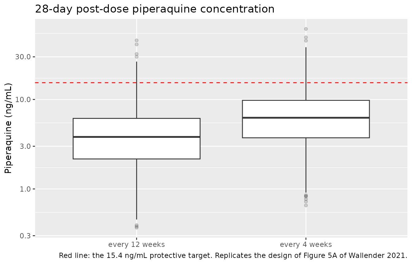
Simulated 28-day post-dose piperaquine concentrations by IPT schedule. Compare with Figure 5A of Wallender 2021, which shows the observed distribution.
Trough concentration by age and nutritional status (Figure 6A)
Figure 6A of the paper reports simulated trough concentrations under the clinical trial protocol, stratified by age and by weight-for-age z-score. The published values come from the authors’ 856-child longitudinal demographic dataset, which is not available, so this is a structural comparison rather than a tight gate: the virtual cohort’s weight trajectory crosses the protocol’s dose bands at different ages than the real cohort did, which is enough to move a single age point by a factor of two.
events_6a <- bind_rows(
  make_arm(100, seq(8, 104, by = 4), "WAZ <= -2", id_offset = 2000L,
           waz_mean = -2.5, waz_sd = 0.5, selfadmin = 0L),
  make_arm(100, seq(8, 104, by = 4), "WAZ > -2",  id_offset = 3000L,
           waz_mean =  0.0, waz_sd = 0.5, selfadmin = 0L)
)
stopifnot(!anyDuplicated(unique(events_6a[, c("id", "time", "evid")])))

sim_6a <- rxode2::rxSolve(
  ui[["Wallender_2021_piperaquine"]],
  events = events_6a, keep = "arm", returnType = "data.frame"
) |>
  as_sim_df() |>
  filter(!is.na(Cc)) |>
  mutate(week = round(time / 7))

published_6a <- tibble::tribble(
  ~arm,        ~week, ~published,
  "WAZ <= -2",  16L,  14.204,
  "WAZ <= -2",  28L,   9.2548,
  "WAZ <= -2",  52L,  13.817,
  "WAZ <= -2", 104L,   9.5958,
  "WAZ > -2",   16L,  23.163,
  "WAZ > -2",   28L,  16.549,
  "WAZ > -2",   52L,  16.994,
  "WAZ > -2",  104L,  12.217
)

cmp_6a <- sim_6a |>
  filter(week %in% published_6a$week) |>
  group_by(arm, week) |>
  summarise(simulated = median(Cc), .groups = "drop") |>
  left_join(published_6a, by = c("arm", "week")) |>
  mutate(ratio = simulated / published)

stopifnot(nrow(cmp_6a) == nrow(published_6a), !anyNA(cmp_6a$published))

cmp_6a |>
  mutate(across(c(simulated, published, ratio), \(x) round(x, 2))) |>
  dplyr::rename(
    "Nutritional stratum"    = arm,
    "Age (weeks)"            = week,
    "Simulated median"       = simulated,
    "Wallender 2021 Fig. 6A" = published,
    "Ratio"                  = ratio
  ) |>
knitr::kable(caption = "Median trough piperaquine concentration (ng/mL) under the clinical trial protocol with full adherence, simulated versus the Figure 6A Source Data.")| Nutritional stratum | Age (weeks) | Simulated median | Wallender 2021 Fig. 6A | Ratio |
|---|---|---|---|---|
| WAZ <= -2 | 16 | 11.38 | 14.20 | 0.80 |
| WAZ <= -2 | 28 | 18.41 | 9.25 | 1.99 |
| WAZ <= -2 | 52 | 15.56 | 13.82 | 1.13 |
| WAZ <= -2 | 104 | 9.88 | 9.60 | 1.03 |
| WAZ > -2 | 16 | 15.86 | 23.16 | 0.68 |
| WAZ > -2 | 28 | 29.32 | 16.55 | 1.77 |
| WAZ > -2 | 52 | 20.80 | 16.99 | 1.22 |
| WAZ > -2 | 104 | 12.67 | 12.22 | 1.04 |
# Wide bound: the published values use a different demographic dataset and the
# dose-band crossings differ. Still red if the malnutrition effect on
# bioavailability, the allometry or the maturation term were dropped.
stopifnot(all(cmp_6a$ratio > 0.3), all(cmp_6a$ratio < 3.0))

# The paper's structural claim: trough concentrations FALL as children age,
# because clearance matures faster than the weight-band doses increase, with
# the lowest troughs after 22 months. Asserted as a magnitude, not a
# step-by-step ordering.
age_trend <- cmp_6a |>
  group_by(arm) |>
  summarise(fall = simulated[week == 104L] / simulated[week == 16L], .groups = "drop")
stopifnot(all(age_trend$fall < 0.95))
Protective efficacy versus piperaquine concentration (Figure 5B)
This is the paper’s central pharmacodynamic result and the strongest gate in this vignette. The Source Data workbook behind Figure 5B tabulates the model-predicted remaining hazard fraction on a 250-point concentration grid; fourteen of those points are transcribed below. The comparison is deterministic (typical values, no cohort), so it is asserted tightly.
Rather than re-typing the Hill equation, the model’s own
protection output is read off a solve and interpolated onto
the published grid. A wrong EC50 or Hill coefficient in
ini() moves it immediately.
mal_typ <- ui[["Wallender_2021_piperaquine_malaria"]] |> rxode2::zeroRe()
#> Warning: some etas defaulted to non-mu referenced, possible parsing error: etaiov_fdepot_1, etaiov_fdepot_2, etaiov_fdepot_3, etaiov_fdepot_4, etaiov_fdepot_5, etaiov_fdepot_6, etaiov_fdepot_7, etaiov_fdepot_8, etaiov_fdepot_9, etaiov_fdepot_10, etaiov_fdepot_11, etaiov_fdepot_12, etaiov_fdepot_13, etaiov_fdepot_14, etaiov_fdepot_15, etaiov_fdepot_16, etaiov_fdepot_17, etaiov_fdepot_18, etaiov_fdepot_19, etaiov_fdepot_20, etaiov_fdepot_21, etaiov_fdepot_22, etaiov_fdepot_23, etaiov_fdepot_24, etaiov_fdepot_25
#> as a work-around try putting the mu-referenced expression on a simple line

# One large dose, then let the concentration decay through the whole published
# range so the model's own concentration-protection pairs can be read off.
sweep_times <- c(seq(0, 5, by = 0.05), seq(5.5, 500, by = 0.5))
events_5b <- data.frame(
  id   = 1L,
  time = c(0, sweep_times),
  amt  = c(320, rep(NA_real_, length(sweep_times))),
  evid = c(1L, rep(0L, length(sweep_times))),
  cmt  = c("depot", rep("central", length(sweep_times))),
  stringsAsFactors = FALSE
)
events_5b$WT <- 8.6
events_5b$PAGE <- 97
events_5b$WAZ <- -0.5
events_5b$SELFADMIN <- 0L
events_5b$OCC <- 0L
events_5b$TRANSM_HIGH_2015 <- 0L
events_5b$TRANSM_HIGH_2016 <- 0L
events_5b$TRANSM_HIGH_2017 <- 0L

sim_5b <- rxode2::rxSolve(mal_typ, events_5b, returnType = "data.frame") |>
  as_sim_df() |>
  filter(!is.na(Cc))
#> ℹ omega/sigma items treated as zero: 'etalcl', 'etalvc', 'etalmtt', 'etaiov_fdepot_1', 'etaiov_fdepot_2', 'etaiov_fdepot_3', 'etaiov_fdepot_4', 'etaiov_fdepot_5', 'etaiov_fdepot_6', 'etaiov_fdepot_7', 'etaiov_fdepot_8', 'etaiov_fdepot_9', 'etaiov_fdepot_10', 'etaiov_fdepot_11', 'etaiov_fdepot_12', 'etaiov_fdepot_13', 'etaiov_fdepot_14', 'etaiov_fdepot_15', 'etaiov_fdepot_16', 'etaiov_fdepot_17', 'etaiov_fdepot_18', 'etaiov_fdepot_19', 'etaiov_fdepot_20', 'etaiov_fdepot_21', 'etaiov_fdepot_22', 'etaiov_fdepot_23', 'etaiov_fdepot_24', 'etaiov_fdepot_25', 'etalhaz_base'

# Terminal decay phase only, so concentration is a monotone index.
decay <- sim_5b |>
  filter(time > time[which.max(Cc)]) |>
  arrange(Cc)
stopifnot(nrow(decay) > 100, min(decay$Cc) < 0.5, max(decay$Cc) > 25)

published_5b <- tibble::tribble(
  ~concentration, ~hazard_fraction,
   0.501, 0.99953385,
   1.001, 0.99600209,
   2.001, 0.96691010,
   3.001, 0.89294402,
   4.001, 0.77370535,
   5.001, 0.63141155,
   6.001, 0.49262937,
   8.001, 0.28485694,
  10.001, 0.16645472,
  12.001, 0.10194591,
  15.401, 0.04959582,
  18.001, 0.03118361,
  21.001, 0.01959185,
  24.901, 0.01161279
)

cmp_5b <- published_5b |>
  mutate(
    model    = 1 - approx(decay$Cc, decay$protection, xout = concentration)$y,
    abs_diff = abs(model - hazard_fraction)
  )
stopifnot(!anyNA(cmp_5b$model))

cmp_5b |>
  mutate(across(c(hazard_fraction, model), \(x) round(x, 5)),
         abs_diff = signif(abs_diff, 3)) |>
  dplyr::rename(
    "Piperaquine (ng/mL)"    = concentration,
    "Wallender 2021 Fig. 5B" = hazard_fraction,
    "Packaged model"         = model,
    "Absolute difference"    = abs_diff
  ) |>
knitr::kable(caption = "Remaining fraction of the malaria hazard. Published values are the median across the paper's 1000 bootstrap parameter draws (Figure 5B Source Data); the model column is the point-estimate prediction, which is why a small systematic difference remains near the EC50.")| Piperaquine (ng/mL) | Wallender 2021 Fig. 5B | Packaged model | Absolute difference |
|---|---|---|---|
| 0.501 | 0.99953 | 0.99958 | 4.47e-05 |
| 1.001 | 0.99600 | 0.99633 | 3.32e-04 |
| 2.001 | 0.96691 | 0.96884 | 1.93e-03 |
| 3.001 | 0.89294 | 0.89737 | 4.43e-03 |
| 4.001 | 0.77371 | 0.78045 | 6.74e-03 |
| 5.001 | 0.63141 | 0.63877 | 7.36e-03 |
| 6.001 | 0.49263 | 0.49988 | 7.25e-03 |
| 8.001 | 0.28486 | 0.28892 | 4.07e-03 |
| 10.001 | 0.16645 | 0.16812 | 1.67e-03 |
| 12.001 | 0.10195 | 0.10269 | 7.41e-04 |
| 15.401 | 0.04960 | 0.04999 | 3.91e-04 |
| 18.001 | 0.03118 | 0.03129 | 1.05e-04 |
| 21.001 | 0.01959 | 0.01943 | 1.59e-04 |
| 24.901 | 0.01161 | 0.01149 | 1.18e-04 |
# Deterministic comparison, so a tight bound is correct. Realised maximum
# 0.0074, entirely at the steep middle of the curve where the bootstrap median
# and the point estimate diverge most. A mis-transcribed EC50 or Hill
# coefficient moves points here by 0.1 or more.
stopifnot(max(cmp_5b$abs_diff) < 0.02)
decay |>
  filter(Cc >= 0.2, Cc <= 25) |>
  ggplot(aes(Cc, protection)) +
  geom_line(linewidth = 0.9) +
  geom_point(
    data = cmp_5b,
    aes(x = concentration, y = 1 - hazard_fraction),
    colour = "red", size = 2
  ) +
  geom_vline(xintercept = 15.4, linetype = "dashed", colour = "grey40") +
  geom_hline(yintercept = 0.95, linetype = "dashed", colour = "grey40") +
  labs(
    x = "Piperaquine (ng/mL)", y = "Fractional reduction in malaria hazard",
    title = "Piperaquine exposure-response for malaria protection",
    caption = "Dashed lines mark the paper's 15.4 ng/mL / 95% protective target."
  )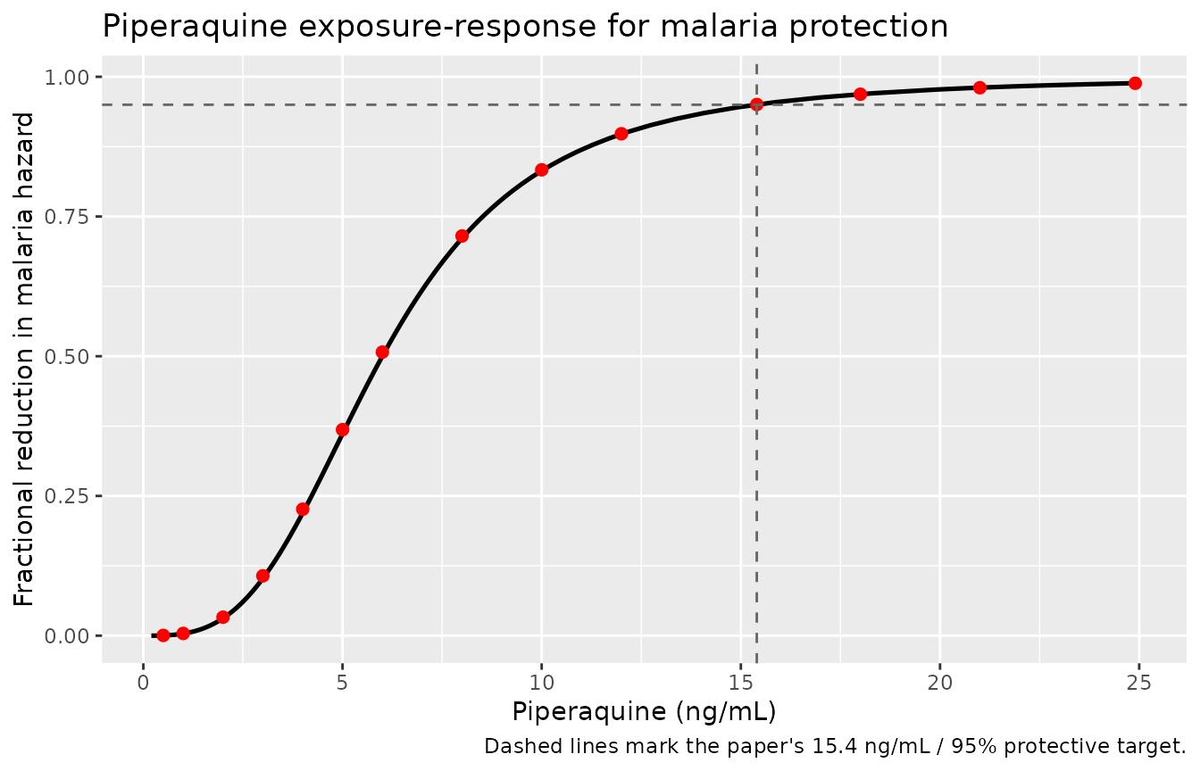
Protective efficacy against incident malaria as a function of piperaquine concentration. Line: packaged model. Points: Figure 5B Source Data of Wallender 2021. Replicates Figure 5B.
The headline claim of the paper is that 15.4 ng/mL reduces the malaria hazard by 95%. That number is over-determined by the two printed Hill parameters, so it is an exact check on both.
protection_at_target <- approx(decay$Cc, decay$protection, xout = 15.4)$y
cat(sprintf(
  "Model hazard reduction at 15.4 ng/mL: %.4f (Wallender 2021: 0.95)\n",
  protection_at_target
))
#> Model hazard reduction at 15.4 ng/mL: 0.9500 (Wallender 2021: 0.95)
stopifnot(abs(protection_at_target - 0.95) < 0.005)
Cumulative malaria risk after a DP course
The paper reports an observed cumulative malaria risk of 8% (6.7-9.3%) through 84 days after a course in the every-12-weeks arm, and 0.1% (0.0-0.30%) through 28 days after a course in the every-4-weeks arm. The observed 8% pools low- and high-transmission calendar periods, so the model is evaluated at both extremes to show that it brackets the published value.
risk_after_course <- function(t2015, t2016, t2017, label) {
  tt <- seq(0, 84, by = 0.25)
  ev <- data.frame(
    id   = 1L,
    time = c(0, 1, 2, tt),
    amt  = c(160, 160, 160, rep(NA_real_, length(tt))),
    evid = c(1L, 1L, 1L, rep(0L, length(tt))),
    cmt  = c(rep("depot", 3), rep("central", length(tt))),
    stringsAsFactors = FALSE
  )
  ev$WT <- 8.6; ev$PAGE <- 97; ev$WAZ <- -0.5
  ev$SELFADMIN <- 1L; ev$OCC <- 1L
  ev$TRANSM_HIGH_2015 <- t2015
  ev$TRANSM_HIGH_2016 <- t2016
  ev$TRANSM_HIGH_2017 <- t2017
  s <- rxode2::rxSolve(mal_typ, ev, returnType = "data.frame") |>
    as_sim_df() |>
    filter(!is.na(Cc))
  tibble(
    period      = label,
    risk_28_day = 1 - exp(-approx(s$time, s$cumhaz, 28)$y),
    risk_84_day = 1 - exp(-approx(s$time, s$cumhaz, 84)$y)
  )
}

risks <- bind_rows(
  risk_after_course(0L, 0L, 0L, "low transmission (reference)"),
  risk_after_course(0L, 1L, 0L, "2016 high transmission"),
  risk_after_course(0L, 0L, 1L, "2017 high transmission")
)
#> ℹ omega/sigma items treated as zero: 'etalcl', 'etalvc', 'etalmtt', 'etaiov_fdepot_1', 'etaiov_fdepot_2', 'etaiov_fdepot_3', 'etaiov_fdepot_4', 'etaiov_fdepot_5', 'etaiov_fdepot_6', 'etaiov_fdepot_7', 'etaiov_fdepot_8', 'etaiov_fdepot_9', 'etaiov_fdepot_10', 'etaiov_fdepot_11', 'etaiov_fdepot_12', 'etaiov_fdepot_13', 'etaiov_fdepot_14', 'etaiov_fdepot_15', 'etaiov_fdepot_16', 'etaiov_fdepot_17', 'etaiov_fdepot_18', 'etaiov_fdepot_19', 'etaiov_fdepot_20', 'etaiov_fdepot_21', 'etaiov_fdepot_22', 'etaiov_fdepot_23', 'etaiov_fdepot_24', 'etaiov_fdepot_25', 'etalhaz_base'
#> ℹ omega/sigma items treated as zero: 'etalcl', 'etalvc', 'etalmtt', 'etaiov_fdepot_1', 'etaiov_fdepot_2', 'etaiov_fdepot_3', 'etaiov_fdepot_4', 'etaiov_fdepot_5', 'etaiov_fdepot_6', 'etaiov_fdepot_7', 'etaiov_fdepot_8', 'etaiov_fdepot_9', 'etaiov_fdepot_10', 'etaiov_fdepot_11', 'etaiov_fdepot_12', 'etaiov_fdepot_13', 'etaiov_fdepot_14', 'etaiov_fdepot_15', 'etaiov_fdepot_16', 'etaiov_fdepot_17', 'etaiov_fdepot_18', 'etaiov_fdepot_19', 'etaiov_fdepot_20', 'etaiov_fdepot_21', 'etaiov_fdepot_22', 'etaiov_fdepot_23', 'etaiov_fdepot_24', 'etaiov_fdepot_25', 'etalhaz_base'
#> ℹ omega/sigma items treated as zero: 'etalcl', 'etalvc', 'etalmtt', 'etaiov_fdepot_1', 'etaiov_fdepot_2', 'etaiov_fdepot_3', 'etaiov_fdepot_4', 'etaiov_fdepot_5', 'etaiov_fdepot_6', 'etaiov_fdepot_7', 'etaiov_fdepot_8', 'etaiov_fdepot_9', 'etaiov_fdepot_10', 'etaiov_fdepot_11', 'etaiov_fdepot_12', 'etaiov_fdepot_13', 'etaiov_fdepot_14', 'etaiov_fdepot_15', 'etaiov_fdepot_16', 'etaiov_fdepot_17', 'etaiov_fdepot_18', 'etaiov_fdepot_19', 'etaiov_fdepot_20', 'etaiov_fdepot_21', 'etaiov_fdepot_22', 'etaiov_fdepot_23', 'etaiov_fdepot_24', 'etaiov_fdepot_25', 'etalhaz_base'

risks |>
  mutate(across(c(risk_28_day, risk_84_day), \(x) round(100 * x, 2))) |>
  dplyr::rename(
    "Transmission period"      = period,
    "Risk through 28 days (%)" = risk_28_day,
    "Risk through 84 days (%)" = risk_84_day
  ) |>
knitr::kable(caption = "Model-predicted cumulative risk of incident malaria after one DP course, typical child, self-administered course. Wallender 2021 reports an observed 8% through 84 days in the every-12-weeks arm, pooled across transmission periods.")| Transmission period | Risk through 28 days (%) | Risk through 84 days (%) |
|---|---|---|
| low transmission (reference) | 0.52 | 2.66 |
| 2016 high transmission | 2.67 | 13.09 |
| 2017 high transmission | 3.99 | 19.05 |
# Deterministic. The observed 8% must sit between the low-transmission and the
# high-transmission predictions, which is the whole point of the transmission
# multipliers. Bounds are wide enough to survive rounding but go red on a
# baseline hazard that is wrong by an order of magnitude (the /1000 scaling).
low  <- risks$risk_84_day[risks$period == "low transmission (reference)"]
high <- risks$risk_84_day[risks$period == "2016 high transmission"]
stopifnot(low < 0.08, high > 0.08, high > 3 * low)

# Protection is strongest early: the risk accrued in the first 28 days after a
# course is a small share of the 84-day total.
stopifnot(all(risks$risk_28_day / risks$risk_84_day < 0.35))
The paper’s every-4-weeks result is much lower still (0.1% through 28 days) because those children never left protective concentrations: each new course arrives on top of the residual from the previous one. The single-course calculation above starts from zero piperaquine, so it is an upper bound on the 28-day risk under a maintained every-4-weeks schedule.
Concentration-QTc relationship
qtc_typ <- ui[["Wallender_2021_piperaquine_qtc"]] |> rxode2::zeroRe()
#> Warning: some etas defaulted to non-mu referenced, possible parsing error: etaiov_fdepot_1, etaiov_fdepot_2, etaiov_fdepot_3, etaiov_fdepot_4, etaiov_fdepot_5, etaiov_fdepot_6, etaiov_fdepot_7, etaiov_fdepot_8, etaiov_fdepot_9, etaiov_fdepot_10, etaiov_fdepot_11, etaiov_fdepot_12, etaiov_fdepot_13, etaiov_fdepot_14, etaiov_fdepot_15, etaiov_fdepot_16, etaiov_fdepot_17, etaiov_fdepot_18, etaiov_fdepot_19, etaiov_fdepot_20, etaiov_fdepot_21, etaiov_fdepot_22, etaiov_fdepot_23, etaiov_fdepot_24, etaiov_fdepot_25
#> as a work-around try putting the mu-referenced expression on a simple line
tt <- seq(0, 28, by = 0.02)
events_qtc <- data.frame(
  id   = 1L,
  time = c(0, 1, 2, tt),
  amt  = c(320, 320, 320, rep(NA_real_, length(tt))),
  evid = c(1L, 1L, 1L, rep(0L, length(tt))),
  cmt  = c(rep("depot", 3), rep("central", length(tt))),
  stringsAsFactors = FALSE
)
events_qtc$WT <- 8.6; events_qtc$PAGE <- 97; events_qtc$WAZ <- -0.5
events_qtc$SELFADMIN <- 0L; events_qtc$OCC <- 1L

sim_qtc <- rxode2::rxSolve(qtc_typ, events_qtc, returnType = "data.frame") |>
  as_sim_df() |>
  filter(!is.na(Cc), Cc > 0)
#> ℹ omega/sigma items treated as zero: 'etalcl', 'etalvc', 'etalmtt', 'etaiov_fdepot_1', 'etaiov_fdepot_2', 'etaiov_fdepot_3', 'etaiov_fdepot_4', 'etaiov_fdepot_5', 'etaiov_fdepot_6', 'etaiov_fdepot_7', 'etaiov_fdepot_8', 'etaiov_fdepot_9', 'etaiov_fdepot_10', 'etaiov_fdepot_11', 'etaiov_fdepot_12', 'etaiov_fdepot_13', 'etaiov_fdepot_14', 'etaiov_fdepot_15', 'etaiov_fdepot_16', 'etaiov_fdepot_17', 'etaiov_fdepot_18', 'etaiov_fdepot_19', 'etaiov_fdepot_20', 'etaiov_fdepot_21', 'etaiov_fdepot_22', 'etaiov_fdepot_23', 'etaiov_fdepot_24', 'etaiov_fdepot_25', 'etale0_qtc'

# The paper's stated effect size: 4.6 msec per 100 ng/mL. Deterministic, so
# asserted tightly; the model slope is 100 * 0.0463 = 4.63.
slope_per_100 <- 100 * with(sim_qtc, coef(lm(dQTcB ~ 0 + Cc))[["Cc"]])
cat(sprintf(
  "Model QTcB increase per 100 ng/mL: %.3f msec (Wallender 2021: 4.6 msec)\n",
  slope_per_100
))
#> Model QTcB increase per 100 ng/mL: 4.630 msec (Wallender 2021: 4.6 msec)
stopifnot(abs(slope_per_100 - 4.6) < 0.1)

cat(sprintf(
  "Peak QTcB after a 320 mg course: %.1f msec (pre-dose baseline %.0f msec)\n",
  max(sim_qtc$QTcB), exp(qtc_typ$theta[["le0_qtc"]])
))
#> Peak QTcB after a 320 mg course: 435.4 msec (pre-dose baseline 410 msec)
sim_qtc |>
  filter(time <= 10) |>
  ggplot(aes(time, QTcB)) +
  geom_line(linewidth = 0.9) +
  labs(
    x = "Time (days)", y = "QTcB (msec)",
    title = "Concentration-driven QTcB after a DP course",
    caption = "Linear concentration effect, 0.0463 msec per ng/mL on a 410 msec pre-dose baseline."
  )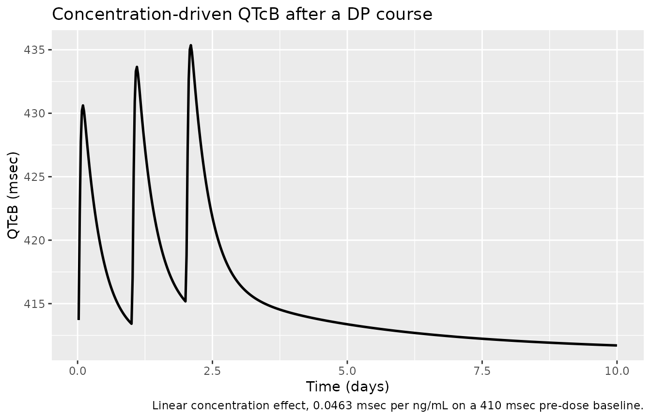
Simulated Bazett-corrected QT interval after a three-day 320 mg piperaquine course, typical child. Replicates the structure of Supplementary Figure 4 of Wallender 2021.
The observed post-drug QTcB in the substudy had a median of 424 msec (range 388-482) against a pre-drug median of 413 msec, which brackets the peak the model predicts for a typical child. The authors caution that peak concentrations under the WHO 2015 and proposed age-based regimens exceed the concentration range this linear model was fitted over, so extrapolating it to those regimens overpredicts QTc prolongation.
PKNCA validation
Wallender 2021 reports no non-compartmental analysis, so there is no
published NCA table to compare against. PKNCA is used here instead as an
independent check that the packaged ODE system, the transit absorption
chain, the bioavailability model and the ng/mL unit scaling compose to
the clearance the paper reports: for a single dose,
AUC(0-inf) must equal dose * F / CL.
n_nca <- 150L
subj_nca <- tibble(
  id  = 5000L + seq_len(n_nca),
  arm = "160 mg single dose",
  WAZ = rnorm(n_nca, -0.5, 1.09)
)
obs_times <- c(seq(0, 3, by = 0.02), seq(3.1, 100, by = 0.2))
events_nca <- bind_rows(
  subj_nca |> mutate(time = 0, amt = 160, evid = 1L, cmt = "depot"),
  subj_nca |> tidyr::crossing(time = obs_times) |>
    mutate(amt = NA_real_, evid = 0L, cmt = "central")
) |>
  mutate(WT = 8.6, PAGE = 97, SELFADMIN = 0L, OCC = 1L, SAMPLE_CAPILLARY = 0L) |>
  arrange(id, time, desc(evid)) |>
  as.data.frame()

sim_nca_raw <- rxode2::rxSolve(
  ui[["Wallender_2021_piperaquine"]],
  events = events_nca, keep = "arm", returnType = "data.frame"
) |>
  as_sim_df()

# Individual CL and F as the model computed them, one row per subject.
per_subject <- sim_nca_raw |>
  group_by(id) |>
  summarise(cl = first(cl), fdepot = first(fdepot), .groups = "drop")
sim_nca <- sim_nca_raw |>
  filter(!is.na(Cc)) |>
  # Per subject, keep Cc >= 1e-6 of Cmax after the peak: below that the ODE tail is solver noise.
  group_by(id) |>
  filter(time <= time[which.max(Cc)] | Cc >= 1e-6 * max(Cc)) |>
  ungroup() |>
  select(id, time, Cc, arm)

# Guarantee a time-zero row per subject; for extravascular dosing Cc = 0
# pre-dose is the correct value.
sim_nca <- bind_rows(
  sim_nca,
  sim_nca |> distinct(id, arm) |> mutate(time = 0, Cc = 0)
) |>
  distinct(id, arm, time, .keep_all = TRUE) |>
  arrange(id, arm, time)

stopifnot(all(sim_nca$Cc >= 0))

conc_obj <- PKNCA::PKNCAconc(sim_nca, Cc ~ time | arm + id)

dose_df <- events_nca |>
  filter(evid == 1L) |>
  select(id, time, amt, arm)
dose_obj <- PKNCA::PKNCAdose(dose_df, amt ~ time | arm + id)

intervals <- data.frame(
  start      = 0,
  end        = Inf,
  cmax       = TRUE,
  tmax       = TRUE,
  aucinf.obs = TRUE,
  half.life  = TRUE
)

nca_res <- PKNCA::pk.nca(PKNCA::PKNCAdata(conc_obj, dose_obj, intervals = intervals))
nca_wide <- as.data.frame(nca_res) |>
  select(id, PPTESTCD, PPORRES) |>
  tidyr::pivot_wider(names_from = PPTESTCD, values_from = PPORRES)

nca_wide |>
  summarise(
    across(c(cmax, tmax, aucinf.obs, half.life),
           list(median = \(x) median(x, na.rm = TRUE),
                p5     = \(x) quantile(x, 0.05, na.rm = TRUE),
                p95    = \(x) quantile(x, 0.95, na.rm = TRUE)))
  ) |>
  tidyr::pivot_longer(everything(), names_to = c("parameter", "stat"),
                      names_pattern = "^(.*)_(median|p5|p95)$") |>
  tidyr::pivot_wider(names_from = stat, values_from = value) |>
  mutate(across(c(median, p5, p95), \(x) signif(x, 4))) |>
  dplyr::rename(
    "NCA parameter" = parameter,
    "Median"        = median,
    "5th pctile"    = p5,
    "95th pctile"   = p95
  ) |>
knitr::kable(caption = "Simulated non-compartmental parameters after a single 160 mg piperaquine dose in a typical 8.6 kg child (Cmax ng/mL, Tmax days, AUC(0-inf) ng*day/mL, half-life days). Wallender 2021 reports no NCA values, so there is no reference column.")| NCA parameter | Median | 5th pctile | 95th pctile |
|---|---|---|---|
| cmax | 244.50 | 74.85 | 768.70 |
| tmax | 0.10 | 0.06 | 0.16 |
| aucinf.obs | 394.80 | 136.70 | 1091.00 |
| half.life | 22.57 | 18.13 | 30.03 |
mass_balance <- nca_wide |>
  left_join(per_subject, by = "id") |>
  mutate(
    # dose 160 mg -> ng: * 1e6; volume L -> mL cancels because CL is L/day and
    # concentration is ng/mL, so dose(mg) * 1e3 / CL(L/day) gives ng*day/mL.
    closed_form = 160 * 1e3 * fdepot / cl,
    rel_diff    = abs(aucinf.obs - closed_form) / closed_form
  )

cat(sprintf(
  "AUC(0-inf) versus dose * F / CL: median relative difference %.4f%%, maximum %.4f%%\n",
  100 * median(mass_balance$rel_diff), 100 * max(mass_balance$rel_diff)
))
#> AUC(0-inf) versus dose * F / CL: median relative difference 0.0131%, maximum 0.0619%

# Deterministic per subject (numerical integration error only), so tight.
stopifnot(max(mass_balance$rel_diff) < 0.02)
Assumptions and deviations
Which Table 2 is final. The Peer Review File distributed with the article contains an earlier revision of Table 2 in which clearance is 435 L/day and age enters as a power function of
(Age / 57 weeks)^0.269. Reviewer 3 asked for a biologically plausible maturation function; the authors refitted with the Emax form and the published Table 2 carries the refitted estimates. Those are the values encoded here. The two agree where they should: the Emax maturation evaluated at the cohort median postmenstrual age of about 97 weeks gives867 * 97 / (97 + 96) = 436L/day, matching the superseded median-centred estimate of 435 L/day.The “1 -” in the hazard equation. Table 2 footnote e abbreviates the survival function without the leading
1 -; Equation 3 in the body carries it. Equation 3 is correct - without it the hazard would rise with drug concentration, inverting the paper’s entire result - and the reading is confirmed arithmetically, since15.4^3.13 / (6.00^3.13 + 15.4^3.13) = 0.9503reproduces the headline 95% hazard reduction. Equation 3 is used.Absorption chain structure. Table 2 gives an “Absorption transit time” of 0.045 day with two pre-specified transit compartments, and the paper never writes the absorption ODEs. The value is read as the mean transit time of the whole chain in the Savic 2007 parameterisation,
ktr = (n + 1) / MTTwithn = 2, givingktr = 66.7per day and a Tmax near 2.3 h. The alternative reading - 0.045 day as a per-compartment time constant,ktr = 22.2per day - changes Cmax by 17% and Tmax by a factor of 2.4 but leaves terminal concentrations, every trough, the 15.4 ng/mL target and the whole malaria hazard layer unchanged to three significant figures. Supplementary Figure 1A was examined specifically to adjudicate this and its x-axis compresses the entire 0.5-8 h intensive-sampling window onto one tick, so observed Tmax cannot settle it. The mean-transit-time reading was confirmed by the maintainers. It matters only for the QTc sub-model, whose output is peak-concentration driven.Slope units in the QTc model. Supplementary Table 2 labels the row “theta Slope /1000 (msec/ng/mL)” with a value of 0.0463, and the body text writes the equation as
+ [PQ] x 0.046/1000. Both are NONMEM estimation-scaling notation relative to the model’s native mg/L concentration unit. The body text pins the effective scale unambiguously - “each 100 ng/mL increase in PPQ concentration was associated with a 4.6 msec increase in the QTcB” - so 0.0463 msec per ng/mL is used directly.Interindividual variability convention. Table 2 and Supplementary Table 2 report variability as %CV. It is converted to the log-normal variance with
omega^2 = log(CV^2 + 1). The paper does not state which convention it used; the alternative (omega^2 = CV^2) would raise the baseline-hazard variance from 0.395 to 0.484.Between-occasion variability. rxode2 has no NONMEM-style
| occvariability level, so the single published BOV term of 66.9% on bioavailability is expanded into 25 per-occasion etas selected by binary indicators on theOCCcolumn, all sharing one variance. Twenty-five covers the every-4-weeks arm exactly. Indicator multiplexing makes rxode2 report “some etas defaulted to non-mu referenced” on every solve; that warning concerns estimation-time mu-referencing optimisations only and is inert for simulation. Simulating more than 25 courses requires adding furtheretaiov_fdepot_<n>terms.No residual error is published for two of the three models. The repeated-time-to-event layer is fitted with an event-density likelihood and Supplementary Table 2 tabulates no residual error for QTcB. Both model files therefore carry a small
fixed()placeholder additive residual, purely so the nlmixr2 likelihood machinery accepts the model for forward simulation. Neither is a published estimate and neither should be read as one.Capillary sampling. The joint venous-plus-capillary fit pooled both matrices into one dependent variable under one proportional residual; separate residual errors were tested and the data did not support them. The PK model therefore predicts the record as drawn, switching between the venous prediction and
Cven^0.922with the per-recordSAMPLE_CAPILLARYindicator. Every simulation in this vignette setsSAMPLE_CAPILLARY = 0, i.e. venous plasma. The capillary conversion is a measurement model, so it is deliberately absent from the two pharmacodynamic model files, which are driven by plasma concentration.QTcBis not a canonical observation name.checkModelConventions()warns that a single-output model should observeCcor a registered PD-output canonical.QTcBis the paper’s own name and matches four QTc models already in the library (QTcS,QTc,QTcI,QTcF); renaming it toCcwould be actively wrong, since it is an ECG interval and not a concentration.Virtual-cohort covariates. Body weight follows a smooth curve pinned to two published values - 3.0 kg at birth (Table 1 median birth weight) and 8.6 kg at 57 weeks (the allometric reference and the cohort median postnatal age) - rather than a WHO growth-standard table, and gestational age is drawn around the Table 1 median of 39.5 weeks. Weight-for-age z-scores are drawn around the cohort median of -0.5 that Equation 2 centres on, with a spread matching the Table 1 percentile range. The Figure 6A comparison uses this curve, whereas the published values come from the authors’ 856-child longitudinal demographic dataset, which is not available; the dose-band crossings therefore fall at different ages, and that is the main reason individual age points in that table differ by up to a factor of two.
Adherence assumption in the Figure 6A comparison. The Figure 6A caption does not state which adherence level it simulated. Full adherence (
SELFADMIN = 0) is assumed there, matching the Figure 6C caption, which does state it. The 28-day trough comparison against the observed data usesSELFADMIN = 1, because only the first of the three daily doses of a routine course was directly observed.Not reproduced. Figure 6B (predicted malaria incidence across simulated baseline transmission intensities) and Table 3 (percentage of time above the protective concentration by regimen, adherence and nutritional status) both depend on the authors’ 856-child longitudinal demographic dataset and on adherence patterns that are described qualitatively rather than parameterised. They are not reproduced here.
No model for the resistance analysis. The pfmdr1 / pfcrt logistic-regression sub-model reports no coefficients, only a null result, so no model file exists for it.