Whole-body PBPK of intravenous iron in mice, rats and humans (Fan 2025) • nlmixr2lib

Model and source

Fan et al. built a 14-compartment perfusion-limited whole-body PBPK model of iron in the mouse, fitted it simultaneously to 13 measured compartments under three dietary iron statuses, and then extrapolated it to the rat and to humans for the iron-carbohydrate complex preparation (IVIP) ferric carboxymaltose (FCM).

Article: https://doi.org/10.1007/s13346-024-01675-x (open access)
Supplement (MOESM1): rat and human physiology tables, the complete NONMEM control stream for the mouse run, and every digitised observed dataset.

The paper contributed five model files, all pointing at this one vignette:

models <- c(
  "Fan_2025_iron_mouse_irondeficient_pbpk",
  "Fan_2025_iron_mouse_ironadequate_pbpk",
  "Fan_2025_iron_mouse_ironloaded_pbpk",
  "Fan_2025_iron_ferriccarboxymaltose_rat_pbpk",
  "Fan_2025_iron_ferriccarboxymaltose_human_pbpk"
)
# readModelDb() returns the model FUNCTION; it must be wrapped in
# rxode2::rxode() before $population / $theta / $state can be read. Calling the
# returned function directly fails with "could not find function 'ini'".
mods <- lapply(models, function(m) rxode2::rxode(readModelDb(m)))
names(mods) <- models
knitr::kable(
  data.frame(
    Model = models,
    Species = vapply(mods, function(u) u$population$species, ""),
    States = vapply(mods, function(u) length(u$state), 0L),
    Endpoints = vapply(mods, function(u) nrow(u$predDf), 0L),
    row.names = NULL
  ),
  caption = "The five packaged models. Three mouse fits (one per dietary iron status), plus the rat and human FCM extrapolations."
)

The five packaged models. Three mouse fits (one per dietary iron status), plus the rat and human FCM extrapolations.
Model	Species	States	Endpoints
Fan_2025_iron_mouse_irondeficient_pbpk	mouse (iron-deficient diet)	14	13
Fan_2025_iron_mouse_ironadequate_pbpk	mouse (iron-adequate diet)	14	13
Fan_2025_iron_mouse_ironloaded_pbpk	mouse (iron-loaded diet)	14	13
Fan_2025_iron_ferriccarboxymaltose_rat_pbpk	rat (Sprague-Dawley, iron-deficiency anaemia)	15	7
Fan_2025_iron_ferriccarboxymaltose_human_pbpk	human (adults with iron-deficiency anaemia)	15	1

cat(mods[[1]]$reference)
#> Fan X, Cao K, Wong RSM, Yan X. A whole-body mechanistic physiologically-based pharmacokinetic modeling of intravenous iron. Drug Deliv Transl Res. 2025;15(3):1109-1120. doi:10.1007/s13346-024-01675-x (PMCID: PMC11870943). The complete NONMEM control stream ($MODEL / $PK / $DES / $ERROR / $THETA / $OMEGA / $SIGMA), the rat and human physiology tables and every digitised observed dataset are in the Electronic Supplementary Material (MOESM1).

Population

The mouse model was fitted to digitised group-mean PK / biodistribution data (reference [23] of the paper). Iron-deficient, iron-adequate and iron-loaded mice were produced by feeding diets of differing iron content, then given a single intravenous bolus of 0.2 umol/kg 59Fe and killed at 15 min, 12 h, 24 h and days 4, 7, 14 and 28. Body weight was 25 g. Only means were available, so the authors used a naive pooled-data method, treating all observations as one individual; consequently no between-subject variability was estimated (all seven $OMEGA elements are 0 FIX) and the packaged models carry no etas.

The rat cohort (reference [24]) had iron-deficiency anaemia and received a single 30 mg Fe/kg IV dose of FCM (345 g body weight). The human cohort (reference [25]) were patients with iron-deficiency anaemia given single ascending IV FCM doses of 100, 500, 800 and 1000 mg Fe; human physiology was fixed to a 73 kg adult.

str(mods[["Fan_2025_iron_mouse_ironadequate_pbpk"]]$population)
#> List of 7
#>  $ species      : chr "mouse (iron-adequate diet)"
#>  $ n_subjects   : chr "not reported; digitised group mean data only"
#>  $ n_studies    : num 1
#>  $ weight_range : chr "25 g (single body weight used for all physiology)"
#>  $ disease_state: chr "Iron-adequate dietary iron status induced by diet"
#>  $ dose_range   : chr "single 0.2 umol/kg 59Fe intravenous bolus (5 nmol in a 25 g mouse)"
#>  $ notes        : chr "Source PK / biodistribution study is reference [23] of the paper; mice were killed and dissected at 15 min, 12 "| __truncated__

Source trace

Every ini() entry carries an in-file comment naming its source location. The table below collects them.

Equation / parameter	Value	Source location
Perfusion-limited organ, `d/dt(<organ>)`	n/a	Eq. (1), p. 1112
Bone, minus erythropoietic utilisation	n/a	Eq. (2), p. 1112
Red-cell pool, `d/dt(rbc_iron)`	n/a	Eq. (3), p. 1112
Spleen, erythrophagocytic return	n/a	Eq. (4), p. 1113
Liver, portal return from gut + spleen	n/a	Eq. (5), p. 1113
Plasma / arterial	n/a	Eq. (6), p. 1113
Residual error, proportional / additive	n/a	Eqs. (7) and (8), p. 1114
`QE(human)` RBC-lifespan allometry	b = 0.75	Eq. (9), p. 1114
Full ODE system as fitted	n/a	Supplement, NONMEM `$DES`
`kp_*` (12 organs), mouse	Table 2	Table 2, p. 1115
`cl` (`CLloss`), mouse	Table 2	Table 2, p. 1115
`q_bone_rbc` (`QE`), mouse	Table 2	Table 2, p. 1115
`mtt_rbc` (`TRBC`), mouse	Table 2	Table 2, p. 1115
Mouse organ volumes / blood flows	Table 1	Table 1, p. 1111 and `$PK`
Mouse cardiac output	`0.275 * BW^0.75` L/min	`$PK` (Brown 1988)
`kp_*` estimated in the rat (6 organs)	8.64, 59.4, 147.9, 17.64, 2.28, 6.41	Results text, p. 1116
Rat organ volumes / blood flows	Supplementary Table 1	Supplement
Human organ volumes / blood flows	Supplementary Table 2	Supplement
`mtt_rbc` (human)	120 days	Methods, p. 1114
Rat / human body weight, cardiac output	0.345 / 73 kg; 6.624 / 336 L/h	Methods, p. 1114
FCM release limb, `KA := q_spleen`	n/a	Methods, p. 1114 (prose only)
Observed datasets (mouse x3, rat, human)	n/a	Supplement, “DATA FILES”

Three ini() values are not printed in the paper and are flagged inline in the model files; see Assumptions and deviations below.

Structural verification

Before comparing against data, two structural properties of the published $DES are checked directly.

u <- mods[["Fan_2025_iron_mouse_ironadequate_pbpk"]]
p <- rxode2::rxSolve(
  u, rxode2::et(amt = 5, cmt = "plasma") |> rxode2::et(c(0, 1)),
  atol = 1e-12, rtol = 1e-10, returnType = "data.frame"
)[1, ]

# The fixed physiology lives in ini(), so it is a PARAMETER: it does not appear
# as a column in the rxSolve output. Only quantities derived inside model()
# (qc, the q_* flows, v_other) come back as columns.
th <- u$theta
fixed_vols <- c("v_bone", "v_gut", "v_heart", "v_kidney", "v_liver", "v_muscle",
                "v_skin", "v_lung", "v_spleen", "v_plasma", "v_adipose",
                "v_brain")

efflux <- with(p, q_other + q_bone + q_heart + q_kidney + q_liver +
                 q_muscle + q_skin + q_brain + q_adipose)
volsum <- sum(th[fixed_vols]) + p$v_other

knitr::kable(data.frame(
  Check = c(
    "Cardiac output (L/h)",
    "Plasma efflux coefficient, excluding cl (L/h)",
    "Efflux / cardiac output",
    "Sum of all 13 compartment volumes (L)",
    "Declared total body volume v_body (L)"
  ),
  Value = c(
    sprintf("%.5f", p$qc), sprintf("%.5f", efflux),
    sprintf("%.10f", efflux / p$qc), sprintf("%.5f", volsum),
    sprintf("%.5f", th[["v_body"]])
  )
), caption = "Plasma mass balance. The efflux coefficient of Eq. (6) equals the cardiac output exactly, and the 13 volumes reconstitute the declared body volume, confirming the rest-of-body derivation used here.")

Plasma mass balance. The efflux coefficient of Eq. (6) equals the cardiac output exactly, and the 13 volumes reconstitute the declared body volume, confirming the rest-of-body derivation used here.
Check	Value
Cardiac output (L/h)	1.03738
Plasma efflux coefficient, excluding cl (L/h)	1.03738
Efflux / cardiac output	1.0000000000
Sum of all 13 compartment volumes (L)	0.03260
Declared total body volume v_body (L)	0.03260

The plasma compartment balances to the cardiac output exactly, which is the evidence that q_other must be computed without subtracting gut and spleen a second time (they are already inside q_liver). Table 1’s printed Remainder blood flow of 0.176 L/h does subtract them twice; see the Errata.

The lung is a different matter. Reproduced verbatim from $DES, it draws the full cardiac output out of plasma and returns nothing, yet q_lung appears in neither the plasma efflux sum nor the plasma influx sum:

cat(sprintf(
  "q_lung = %.5f L/h, but q_lung is absent from the plasma ODE.\n%s\n",
  p$q_lung,
  "The lung is therefore a non-mass-balanced observer compartment as published."
))
#> q_lung = 1.03738 L/h, but q_lung is absent from the plasma ODE.
#> The lung is therefore a non-mass-balanced observer compartment as published.

This is kept as fitted rather than silently corrected, because the Table 2 partition coefficients were estimated against exactly this system.

Mouse: reproducing Figures 3 and 4

The observed data are the digitised group means transcribed in the supplement’s “DATA FILES” section, in nmol of 59Fe. Note that the supplement tabulates times in days while the model’s rate constants are per hour, so the observation times are multiplied by 24.

mouse_obs <- bind_rows(
  data.frame(diet = "iron-deficient", time = c(0.5, 1, 4, 7, 14, 28),
    plasma = c(.1088,.05576,.02312,.02312,.01632,.02312),
    bone = c(1.8954,.3978,.297,.1728,.0738,.1152),
    gut = c(.44894,.29366,.2344,.13146,.07906,.06134),
    heart = c(.0462,.0378,.0518,.0462,.0364,.0574),
    kidney = c(.1368,.1102,.1368,.057,.057,.0722),
    liver = c(.68198,.60268,.65758,.31598,.2806,.13176),
    muscle = c(.4026,.5368,.4026,.4026,.2684,.671),
    skin = c(.0124,.0186,.0155,.0186,.0124,.0093),
    lung = c(.1157,.338,.1586,.0364,.0624,.0208),
    spleen = c(.09079,.03017,.00595,NA,NA,NA),
    rbc_iron = c(.6248,1.42,1.8744,1.9312,2.0732,1.9596),
    brain = c(.0094,.0094,.0141,.0188,.0188,.0188),
    adipose = c(.0124,.0186,.0155,.0186,.0124,.0093)),
  data.frame(diet = "iron-adequate", time = c(0.5, 1, 4, 7, 14, 28),
    plasma = c(.11832,.0204,.01496,.0068,.01768,.02176),
    bone = c(3.4866,1.296,.6858,.5076,.4518,.2232),
    gut = c(.4514,.366,.1952,.061,.0488,.0366),
    heart = c(.0728,.0364,.056,.056,.0518,.0322),
    kidney = c(.19,.1178,.133,.0646,.0646,.0684),
    liver = c(1.03578,.86132,.81008,.66734,.52704,.31476),
    muscle = c(.8052,.4026,.4026,1.0736,.1342,.2684),
    skin = c(.5955,.397,.5558,.5955,.7146,.2779),
    lung = c(.1014,.1521,.0637,.0429,.0429,.039),
    spleen = c(.05817,.08071,.04333,.04074,.02786,.03066),
    rbc_iron = c(.6106,1.2283,1.5762,1.2638,1.2496,1.1644),
    brain = c(.0141,.0094,.0141,.0094,.0141,.0094),
    adipose = c(.0124,.0186,.0155,.0341,.0155,.0031)),
  data.frame(diet = "iron-loaded", time = c(0.5, 1, 4, 7, 14, 28),
    plasma = c(.1156,.03536,.00816,.00544,.00952,.01768),
    bone = c(1.9116,1.2348,.4212,.3438,.5472,.3168),
    gut = c(.28426,.47214,.20374,.10126,.09394,.07686),
    heart = c(.0938,.1134,.0896,.1036,.042,.0378),
    kidney = c(.285,.646,.38,.1786,.1558,.133),
    liver = c(.93818,2.84504,1.8361,1.0248,1.0919,1.09556),
    muscle = c(.5368,1.0736,.5368,.5368,.5368,.2684),
    skin = c(.397,.794,.3176,.397,.3573,.3573),
    lung = c(.1833,.1742,.1898,.3965,.1638,.104),
    spleen = c(.03682,.06902,.04431,.04963,.04424,.06496),
    rbc_iron = c(.1704,.3692,.568,.852,1.3064,.9088),
    brain = c(.0047,.0094,.0047,.0094,.0141,.0094),
    adipose = c(.0124,.0279,.0186,.0217,.0217,.0062))
) |>
  pivot_longer(-c(diet, time), names_to = "compartment", values_to = "obs") |>
  filter(!is.na(obs)) |>
  mutate(time_h = time * 24)

diet_model <- c(
  "iron-deficient" = "Fan_2025_iron_mouse_irondeficient_pbpk",
  "iron-adequate"  = "Fan_2025_iron_mouse_ironadequate_pbpk",
  "iron-loaded"    = "Fan_2025_iron_mouse_ironloaded_pbpk"
)

mouse_sim <- bind_rows(lapply(names(diet_model), function(d) {
  ev <- rxode2::et(amt = 5, cmt = "plasma") |> rxode2::et(seq(0, 672, by = 4))
  s <- rxode2::rxSolve(mods[[diet_model[[d]]]], ev,
                       atol = 1e-12, rtol = 1e-10, returnType = "data.frame")
  s |>
    select(time, all_of(unique(mouse_obs$compartment))) |>
    pivot_longer(-time, names_to = "compartment", values_to = "pred") |>
    mutate(diet = d)
}))

ggplot(mouse_sim, aes(time / 24, pred, colour = diet)) +
  geom_line() +
  geom_point(data = mouse_obs, aes(time, obs, colour = diet), size = 1.1) +
  facet_wrap(~compartment, scales = "free_y", ncol = 4) +
  scale_x_continuous(breaks = c(0, 7, 14, 21, 28)) +
  labs(x = "Time (days)", y = "59Fe amount (nmol)", colour = "Diet") +
  theme_bw(base_size = 9) +
  theme(legend.position = "top")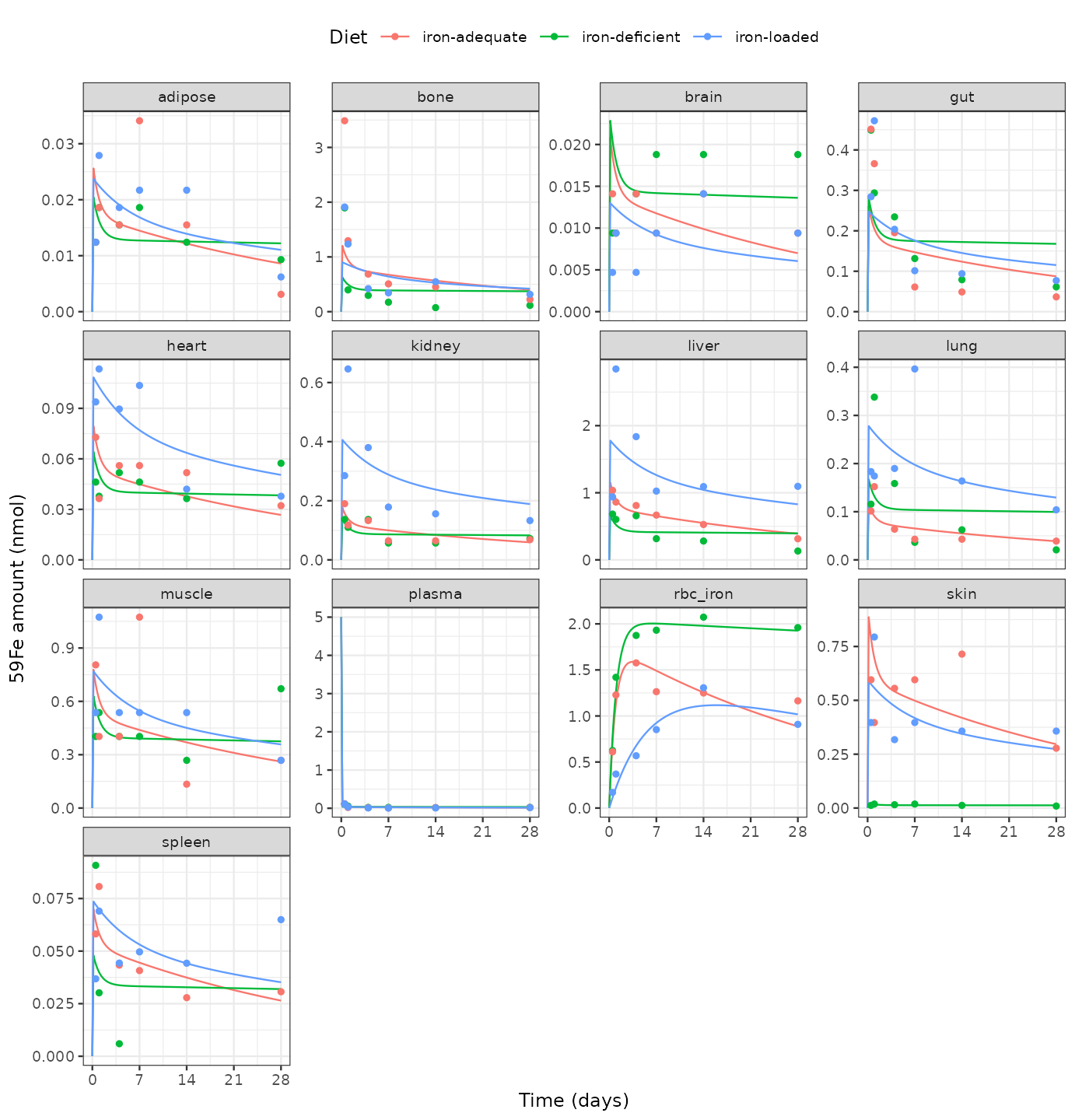

Replicates Figures 3 and 4 of Fan 2025: observed (points, digitised group means) and model-predicted (lines) 59Fe amounts in plasma and 12 tissues after a single 0.2 umol/kg IV bolus, under three dietary iron statuses.

# Interpolate per (diet, compartment) group. Deliberately NOT a left_join:
# mouse_obs and mouse_sim both carry a `time` column, so a join renames them to
# time.x / time.y and a bare `time` inside approx() would silently resolve to
# stats::time() instead of the data.
mouse_cmp <- do.call(rbind, lapply(
  split(mouse_obs, list(mouse_obs$diet, mouse_obs$compartment), drop = TRUE),
  function(o) {
    s <- mouse_sim[mouse_sim$diet == o$diet[1] &
                     mouse_sim$compartment == o$compartment[1], ]
    o$pred <- approx(s$time, s$pred, xout = o$time_h)$y
    o
  }
))
mouse_cmp$ratio <- mouse_cmp$pred / mouse_cmp$obs
stopifnot(nrow(mouse_cmp) == nrow(mouse_obs), !anyNA(mouse_cmp$pred))

knitr::kable(
  mouse_cmp |>
    group_by(Diet = diet) |>
    summarise(
      n = n(),
      `Geometric mean pred/obs` = sprintf("%.3f", exp(mean(log(ratio)))),
      `Mean |log10 ratio|` = sprintf("%.3f", mean(abs(log10(ratio)))),
      `Within 2-fold` = sprintf("%.0f%%", 100 * mean(abs(log10(ratio)) < log10(2)))
    ),
  caption = "Mouse model agreement across plasma and 12 tissues. A geometric mean pred/obs near 1 with 80-88% of points inside 2-fold is close agreement for a 13-endpoint simultaneous fit to digitised means."
)

Mouse model agreement across plasma and 12 tissues. A geometric mean pred/obs near 1 with 80-88% of points inside 2-fold is close agreement for a 13-endpoint simultaneous fit to digitised means.
Diet	n	Geometric mean pred/obs	Mean \|log10 ratio\|	Within 2-fold
iron-adequate	78	1.065	0.147	86%
iron-deficient	75	1.145	0.181	80%
iron-loaded	78	1.082	0.158	88%

All three diets reproduce the published fit: the geometric mean predicted / observed ratio is 1.07 to 1.15 and 80-88 % of the 75-78 observations fall inside two-fold. The model also reproduces the paper’s mechanistic conclusions: the iron-deficient fit has the highest q_bone_rbc and the lowest cl, driving 59Fe into the red-cell pool, while the iron-loaded fit has the largest liver, heart and kidney partition coefficients.

knitr::kable(
  data.frame(
    Diet = names(diet_model),
    `q_bone_rbc (L/h)` = sprintf("%.2e", vapply(diet_model, function(m)
      exp(mods[[m]]$theta[["lq_bone_rbc"]]), 0)),
    `cl (L/h)` = sprintf("%.3e", vapply(diet_model, function(m)
      exp(mods[[m]]$theta[["lcl"]]), 0)),
    `kp_liver` = sprintf("%.2f", vapply(diet_model, function(m)
      exp(mods[[m]]$theta[["lkp_liver"]]), 0)),
    `mtt_rbc (h)` = sprintf("%.2f", vapply(diet_model, function(m)
      exp(mods[[m]]$theta[["lmtt_rbc"]]), 0)),
    row.names = NULL, check.names = FALSE
  ),
  caption = "Table 2 parameters that carry the paper's mechanistic argument, read back from the packaged models."
)

Table 2 parameters that carry the paper’s mechanistic argument, read back from the packaged models.
Diet	q_bone_rbc (L/h)	cl (L/h)	kp_liver	mtt_rbc (h)
iron-deficient	4.34e-04	1.240e-05	9.38	41.53
iron-adequate	2.17e-04	1.647e-04	18.11	34.44
iron-loaded	3.88e-05	1.184e-04	38.53	197.60

Rat: reproducing Figure 5

The rat and human models add one circulating ivip compartment: the whole IV FCM dose lands there and is taken up by splenic macrophages at a rate set equal to the spleen blood flow (KA := q_spleen). Observations are on total serum iron, Cc = (plasma + ivip) / v_plasma.

Both extrapolation models declare several endpoints, so observation records must identify which endpoint they belong to. dvid = 1 selects the first endpoint (Cc); this is the dvid() route rather than writing cmt = "Cc", which would reference an algebraic observable as if it were a compartment.

ev_ivip <- function(dose, times) {
  # Keep t = 0 in the observation grid. The dose record comes first, so the
  # t = 0 observation reports the POST-dose state and Cc(0) = dose / v_plasma
  # exactly -- which is the dose-to-serum mapping check used below. Dropping
  # t = 0 silently loses that row and makes the mapping table empty.
  times <- sort(unique(c(0, times[times >= 0])))
  data.frame(
    id   = 1L,
    time = c(0, times),
    amt  = c(dose, rep(NA_real_, length(times))),
    evid = c(1L, rep(0L, length(times))),
    cmt  = c("ivip", rep(NA_character_, length(times))),
    dvid = c(NA_integer_, rep(1L, length(times)))
  )
}

rat_serum <- data.frame(
  time = c(1, 2, 4, 6, 8, 12, 24, 48),
  obs = c(1147.87, 979.73, 625.86, 839.33, 660.93, 526.43, 438.72, 111.29)
)
rat_tissue <- data.frame(time = c(72, 192, 360),
  Cbone = c(42.40, 38.99, 15.27), Cheart = c(64.54, 51.70, 40.42),
  Ckidney = c(36.65, 25.70, 19.92), Cliver = c(341.36, 236.92, 84.11),
  Cmuscle = c(11.83, 11.27, 7.70), Cspleen = c(449.76, 461.72, 385.17)
) |> pivot_longer(-time, names_to = "compartment", values_to = "obs")

ur <- mods[["Fan_2025_iron_ferriccarboxymaltose_rat_pbpk"]]
sr <- rxode2::rxSolve(
  ur, ev_ivip(10.35, c(seq(0, 400, by = 0.25), rat_serum$time, rat_tissue$time)),
  atol = 1e-12, rtol = 1e-10, returnType = "data.frame"
)

rat_cmp <- bind_rows(
  rat_serum |>
    mutate(compartment = "serum (ug/dL)",
           pred = approx(sr$time, sr$Cc * 100, xout = time)$y),
  rat_tissue |>
    group_by(compartment) |>
    mutate(pred = approx(sr$time, sr[[first(compartment)]], xout = time)$y) |>
    ungroup()
) |> mutate(ratio = pred / obs)

knitr::kable(
  rat_cmp |>
    mutate(Group = if_else(compartment == "serum (ug/dL)", "Serum", "Tissue")) |>
    group_by(Group) |>
    summarise(n = n(),
      `Geometric mean pred/obs` = sprintf("%.2f", exp(mean(log(ratio)))),
      `Mean |log10 ratio|` = sprintf("%.2f", mean(abs(log10(ratio)))),
      `Within 2-fold` = sprintf("%.0f%%", 100 * mean(abs(log10(ratio)) < log10(2)))),
  caption = "Rat extrapolation agreement (Figure 5). Serum is 30 mg Fe/kg FCM; tissues are bone, heart, kidney, liver, muscle and spleen at 72, 192 and 360 h. Read the serum row together with the shape check below -- a good average ratio here does NOT mean the serum profile is reproduced."
)

Rat extrapolation agreement (Figure 5). Serum is 30 mg Fe/kg FCM; tissues are bone, heart, kidney, liver, muscle and spleen at 72, 192 and 360 h. Read the serum row together with the shape check below – a good average ratio here does NOT mean the serum profile is reproduced.
Group	n	Geometric mean pred/obs	Mean \|log10 ratio\|	Within 2-fold
Serum	8	1.10	0.20	75%
Tissue	18	1.42	0.16	89%

A level-agreement statistic is not enough for the serum profile, so the shape is checked separately: how far does each series fall between the first and last serum observation?

rs <- filter(rat_cmp, compartment == "serum (ug/dL)")
knitr::kable(data.frame(
  Series = c("Observed (digitised)", "Predicted"),
  `First (1 h)` = sprintf("%.0f", c(rs$obs[1], rs$pred[1])),
  `Last (48 h)` = sprintf("%.0f", c(rs$obs[nrow(rs)], rs$pred[nrow(rs)])),
  `Fold decline, 1-48 h` = sprintf("%.1f-fold",
    c(rs$obs[1] / rs$obs[nrow(rs)], rs$pred[1] / rs$pred[nrow(rs)])),
  check.names = FALSE
), caption = "Rat serum shape check. The observed profile falls about 10-fold over 1-48 h; the model falls about 1.5-fold. The serum decline is NOT reproduced, and the favourable geometric mean above is a consequence of a near-flat prediction sitting in the middle of a declining observation series.")

Rat serum shape check. The observed profile falls about 10-fold over 1-48 h; the model falls about 1.5-fold. The serum decline is NOT reproduced, and the favourable geometric mean above is a consequence of a near-flat prediction sitting in the middle of a declining observation series.
Series	First (1 h)	Last (48 h)	Fold decline, 1-48 h
Observed (digitised)	1148	111	10.3-fold
Predicted	853	588	1.5-fold

ggplot(data.frame(time = sr$time, pred = sr$Cc * 100), aes(time, pred)) +
  geom_line() +
  geom_point(data = rat_serum, aes(time, obs), size = 1.6) +
  coord_cartesian(xlim = c(0, 60)) +
  labs(x = "Time (h)", y = "Serum iron (ug/dL)") +
  theme_bw(base_size = 10)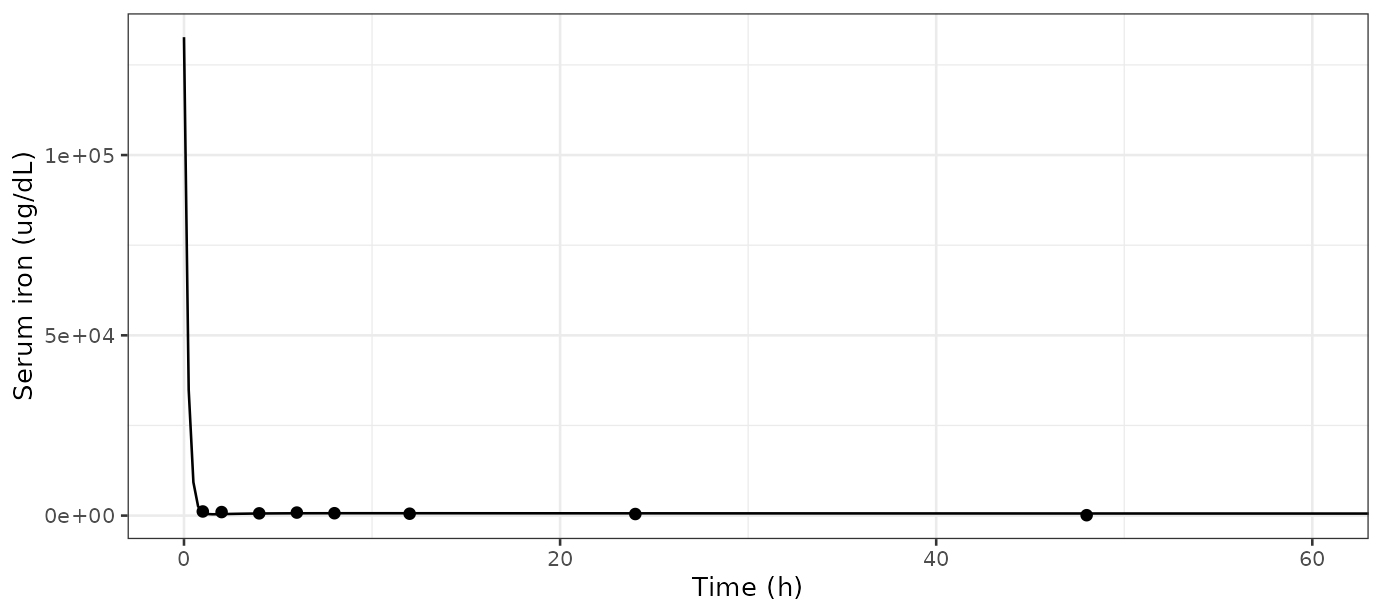

Replicates Figure 5 of Fan 2025: observed (points) and predicted (line) serum iron in iron-deficient rats after a single 30 mg Fe/kg IV dose of ferric carboxymaltose.

The rat tissue distribution is reproduced; the rat serum profile is not.

The six measured tissues sit at a geometric mean predicted / observed ratio of 1.42 with 89 % of points inside two-fold - good agreement, and the substantive result, since tissue burden is what the model exists to predict. The over-prediction is concentrated at the last time point (360 h), consistent with the authors’ own caution about sparse terminal data.

Serum is a different story. The average level is close (geometric mean 1.10), but that number is misleading: KA := q_spleen clears the FCM colloid out of rat serum with a half-life of ln(2) * 0.0078 / 0.0417 = 0.13 h, so more than 99 % of the dose has left the ivip compartment by the first observation at 1 h. From then on serum is set by return flux from the tissues, which is nearly flat. The prediction therefore falls about 1.5-fold over 1-48 h against an observed 10-fold decline, and the good average ratio is an artifact of a flat line crossing a declining one. Unlike the human case below, refitting q_spleen does not repair the rat profile (the implied value is within a few percent of the published one), because the rat serum level is governed by tissue return rather than by colloid release. The authors report only that “the iron concentration in the serum was slightly overestimated to a lesser degree after 20 h”; the discrepancy is in the shape, not the level.

Human: reproducing Figure 6

human_obs <- data.frame(
  time = c(.25,.5,.75,1,1.5,2,3,4,6,8,12,16,24,36,48,60,72),
  `100` = c(36.3,36.1,34.73,33.17,31.69,31.27,26.97,25.50,20.92,17.97,
            13.66,12.59,8.82,7.75,7,NA,NA),
  `500` = c(153.23,150,148.39,141.94,140.32,133.87,127.42,122.58,101.61,88.71,
            69.35,51.61,30.65,12.90,8.06,7,NA),
  `800` = c(287.72,292.61,272.89,287.63,292.47,262.90,285.71,239.67,218.10,
            185.03,141.87,124.93,79.59,29.87,11.57,8.74,7),
  `1000` = c(322.87,NA,308.37,318.46,320.78,308.09,297.72,288.99,261.61,240.79,
             215.71,175.79,135.21,78.74,54.64,22.10,7),
  check.names = FALSE
) |>
  pivot_longer(-time, names_to = "dose", values_to = "obs") |>
  filter(!is.na(obs)) |>
  mutate(dose_mg = as.numeric(dose))

uh <- mods[["Fan_2025_iron_ferriccarboxymaltose_human_pbpk"]]
human_times <- c(human_obs$time, seq(0, 80, by = 0.1))
human_sim <- bind_rows(lapply(c(100, 500, 800, 1000), function(d) {
  s <- rxode2::rxSolve(uh, ev_ivip(d, human_times), atol = 1e-14, rtol = 1e-12,
                       returnType = "data.frame")
  data.frame(time = s$time, pred = s$Cc, dose = as.character(d), dose_mg = d)
}))

ggplot(human_sim, aes(time, pred, colour = dose)) +
  geom_line() +
  geom_point(data = human_obs, aes(time, obs, colour = dose), size = 1.4) +
  scale_y_log10() +
  coord_cartesian(xlim = c(0, 72), ylim = c(1, 500)) +
  labs(x = "Time (h)", y = "Total serum iron (ug/mL)", colour = "Dose (mg)") +
  theme_bw(base_size = 10)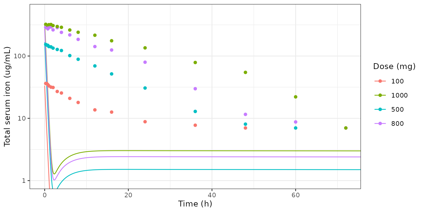

Replicates Figure 6 of Fan 2025: observed (points, digitised) and predicted (lines) total serum iron after single ascending IV doses of ferric carboxymaltose. The predicted peak matches, but the predicted decline is far too fast – see the Errata.

Two distinct checks are needed here, and conflating them is easy. The first asks whether the dose-to-serum mapping is right: does the whole dose show up in the serum volume immediately after the bolus? The second asks whether the model matches the data at the times the data were actually collected, the first of which is 0.25 h.

h0 <- human_sim |> filter(time == 0) |> select(dose_mg, cc0 = pred)
knitr::kable(
  h0 |> transmute(`Dose (mg)` = dose_mg,
                  `dose / v_plasma = dose / 3 L (ug/mL)` = sprintf("%.1f", dose_mg / 3),
                  `Model Cc at t = 0+ (ug/mL)` = sprintf("%.1f", cc0),
                  `Ratio` = sprintf("%.3f", cc0 / (dose_mg / 3))),
  caption = "Dose-to-serum mapping check. Immediately after the bolus the model holds the entire dose in the 3 L serum volume, so Cc(0+) = dose / 3 exactly. This confirms the dosing route and the observation definition, and it is the right order of magnitude for the observed peaks (36-323 ug/mL) -- but t = 0+ is not an observable sample."
)

Dose-to-serum mapping check. Immediately after the bolus the model holds the entire dose in the 3 L serum volume, so Cc(0+) = dose / 3 exactly. This confirms the dosing route and the observation definition, and it is the right order of magnitude for the observed peaks (36-323 ug/mL) – but t = 0+ is not an observable sample.
Dose (mg)	dose / v_plasma = dose / 3 L (ug/mL)	Model Cc at t = 0+ (ug/mL)	Ratio
100	33.3	33.3	1.000
500	166.7	166.7	1.000
800	266.7	266.7	1.000
1000	333.3	333.3	1.000

human_matched <- human_obs |>
  group_by(dose_mg) |>
  group_modify(function(.x, .y) {
    s <- human_sim[human_sim$dose_mg == .y$dose_mg, ]
    .x$pred <- approx(s$time, s$pred, xout = .x$time)$y
    .x
  }) |>
  ungroup() |>
  mutate(ratio = pred / obs)

knitr::kable(
  human_matched |>
    group_by(`Dose (mg)` = dose_mg) |>
    summarise(
      n = n(),
      `Obs at 0.25 h` = sprintf("%.1f", obs[which.min(time)]),
      `Pred at 0.25 h` = sprintf("%.1f", pred[which.min(time)]),
      `Ratio at 0.25 h` = sprintf("%.2f", (pred / obs)[which.min(time)]),
      `Geomean pred/obs, all times` = sprintf("%.3f", exp(mean(log(ratio)))),
      .groups = "drop"
    ),
  caption = "Human serum at MATCHED observation times. Even the earliest sample at 0.25 h is already about 2.2-fold low, and averaged over the whole profile the model is roughly 30-fold low. The peak is NOT reproduced at any sampled time."
)

Human serum at MATCHED observation times. Even the earliest sample at 0.25 h is already about 2.2-fold low, and averaged over the whole profile the model is roughly 30-fold low. The peak is NOT reproduced at any sampled time.
Dose (mg)	n	Obs at 0.25 h	Pred at 0.25 h	Ratio at 0.25 h	Geomean pred/obs, all times
100	15	36.3	14.4	0.40	0.026
500	16	153.2	72.0	0.47	0.039
800	17	287.7	115.1	0.40	0.036
1000	16	322.9	143.9	0.45	0.028

So the dose-to-serum mapping is right, but the profile is not reproduced at any observed time, including the first. The reason is that splenic macrophage uptake is set to the human spleen blood flow, q_spleen = 10.08 L/h, giving an intact-colloid serum half-life of ln(2) * 3 / 10.08 = 0.21 h; by the 0.25 h sample the model has already shed more than half the dose out of serum, and by 1 h it has shed 96 % of it. The observed profiles instead decline with a terminal half-life of roughly 10-15 h. Fitting q_spleen as a free parameter to the 1000 mg profile - a diagnostic only, not a change to the packaged model - recovers the data closely:

h1000 <- filter(human_obs, dose_mg == 1000)
ev1000 <- ev_ivip(1000, c(h1000$time, seq(0, 80, by = 0.25)))
obj <- function(lka) {
  s <- rxode2::rxSolve(uh, c(q_spleen = exp(lka)), ev1000,
                       atol = 1e-12, rtol = 1e-10, returnType = "data.frame")
  sum((log(pmax(approx(s$time, s$Cc, xout = h1000$time)$y, 1e-9)) -
         log(h1000$obs))^2)
}
o <- optimize(obj, c(log(1e-3), log(50)))
sfit <- rxode2::rxSolve(uh, c(q_spleen = exp(o$minimum)), ev1000,
                        atol = 1e-12, rtol = 1e-10, returnType = "data.frame")
rfit <- approx(sfit$time, sfit$Cc, xout = h1000$time)$y / h1000$obs
knitr::kable(data.frame(
  Quantity = c("Published KA := q_spleen (L/h)",
               "Implied effective KA from the 1000 mg profile (L/h)",
               "Ratio", "Geometric mean pred/obs with the implied KA",
               "Mean |log10 ratio| with the implied KA"),
  Value = c("10.08", sprintf("%.3f", exp(o$minimum)),
            sprintf("%.0f-fold slower", 10.08 / exp(o$minimum)),
            sprintf("%.2f", exp(mean(log(rfit)))),
            sprintf("%.2f", mean(abs(log10(rfit)))))
), caption = "Diagnostic only. The structure and the dose-to-serum mapping are correct; the single simplification KA := q_spleen is about 72-fold too fast in humans. The packaged model retains the published value.")

Diagnostic only. The structure and the dose-to-serum mapping are correct; the single simplification KA := q_spleen is about 72-fold too fast in humans. The packaged model retains the published value.
Quantity	Value
Published KA := q_spleen (L/h)	10.08
Implied effective KA from the 1000 mg profile (L/h)	0.139
Ratio	72-fold slower
Geometric mean pred/obs with the implied KA	0.96
Mean \|log10 ratio\| with the implied KA	0.05

So the human file is a faithful encoding of the published recipe, and it is internally consistent and exactly dose-proportional, but it does not reproduce the observed serum time course at any sampled time. This is a property of the paper, not of the extraction; it is recorded in the Errata below.

NCA validation (PKNCA)

The paper reports no NCA table, so the simulated human profiles are compared against NCA of the digitised observed profiles. Both series are put on the same time grid - the actual observation times - and the interval starts at the first measurement (0.25 h), so neither series needs a fabricated time-zero record and PKNCA raises no “AUC range starting before the first measurement” warning. This makes the comparison a direct statement about the profiles rather than about an extrapolation choice.

half.life is deliberately not requested: the simulated profile is non-monotonic (a fast collapse followed by a slow rebound plateau fed by tissue return), so a terminal slope is not a meaningful quantity for it.

nca_frame <- function(df, value) {
  df |>
    transmute(id = 1L, treatment = paste(dose_mg, "mg"), time,
              Cc = .data[[value]]) |>
    filter(!is.na(Cc)) |>
    arrange(treatment, time)
}

run_nca <- function(conc_df, doses) {
  conc_obj <- PKNCA::PKNCAconc(conc_df, Cc ~ time | treatment + id,
                               concu = "ug/mL", timeu = "h")
  dose_obj <- PKNCA::PKNCAdose(doses, amt ~ time | treatment + id,
                               doseu = "mg")
  # tmax is omitted: both series peak at (or one sample after) the first
  # record of an IV bolus profile that starts at 0.25 h, so it carries no
  # information here and PKNCA reports it relative to the interval start.
  intervals <- data.frame(start = min(conc_df$time), end = 48,
                          cmax = TRUE, auclast = TRUE)
  PKNCA::pk.nca(PKNCA::PKNCAdata(conc_obj, dose_obj, intervals = intervals))
}

dose_df <- data.frame(id = 1L, time = 0,
                      amt = c(100, 500, 800, 1000),
                      treatment = paste(c(100, 500, 800, 1000), "mg"))

nca_obs <- run_nca(nca_frame(filter(human_matched, time <= 48), "obs"), dose_df)
nca_sim <- run_nca(nca_frame(filter(human_matched, time <= 48), "pred"), dose_df)

cmp <- nlmixr2lib::ncaComparisonTable(
  simulated = nca_sim,
  reference = nca_obs,
  by = "treatment",
  params = c("cmax", "auclast"),
  units = c(cmax = "ug/mL", auclast = "ug*h/mL"),
  tolerance_pct = 20
)
knitr::kable(
  cmp,
  caption = "Simulated vs digitised-observed NCA of human total serum iron on matched observation times, 0.25-48 h. Every Cmax and AUClast row is starred: the packaged model is roughly 2-fold low at the earliest sample and roughly 25-fold low on exposure. Starred rows differ by more than 20%."
)

Simulated vs digitised-observed NCA of human total serum iron on matched observation times, 0.25-48 h. Every Cmax and AUClast row is starred: the packaged model is roughly 2-fold low at the earliest sample and roughly 25-fold low on exposure. Starred rows differ by more than 20%.
NCA parameter	treatment	Reference	Simulated	% diff
Cmax (ug/mL)	100 mg	36.3	14.4	-60.3%*
Cmax (ug/mL)	1000 mg	323	144	-55.4%*
Cmax (ug/mL)	500 mg	153	72	-53.0%*
Cmax (ug/mL)	800 mg	293	115	-60.6%*
AUClast (ug*h/mL)	100 mg	587	17.7	-97.0%*
AUClast (ug*h/mL)	1000 mg	7180	177	-97.5%*
AUClast (ug*h/mL)	500 mg	2170	88.3	-95.9%*
AUClast (ug*h/mL)	800 mg	4720	141	-97.0%*

Every Cmax and AUClast row is starred. This is the expected, documented consequence of KA := q_spleen (see the Errata), not a signal to tune any parameter. It is recorded here rather than suppressed, because a reader deciding whether to use the human file for an exposure calculation needs to see it.

What the model does get right is strict dose proportionality, which is worth confirming separately since it is the property the file remains usable for:

# Integrate on the COMMON simulation grid, not on the per-dose observed times:
# the four observed series have different sampling schedules and different last
# observed times, so a trapezoid over them is not comparable across doses and
# would not test linearity at all.
dose_prop <- human_sim |>
  filter(time <= 48) |>
  arrange(dose_mg, time) |>
  group_by(dose_mg) |>
  summarise(
    auc = sum(diff(time) * (head(pred, -1) + tail(pred, -1)) / 2),
    .groups = "drop"
  ) |>
  mutate(auc_per_dose = auc / dose_mg)

knitr::kable(
  dose_prop |>
    transmute(`Dose (mg)` = dose_mg,
              `Simulated AUC 0-48 h (ug*h/mL)` = sprintf("%.2f", auc),
              `AUC / dose` = sprintf("%.6f", auc_per_dose)),
  caption = "Simulated exposure on a common 0-48 h grid is exactly proportional to dose (constant AUC / dose), as expected for a linear system dosed into a single serum volume. The model is internally consistent; it is the absolute level of the serum time course that does not match the data."
)

Simulated exposure on a common 0-48 h grid is exactly proportional to dose (constant AUC / dose), as expected for a linear system dosed into a single serum volume. The model is internally consistent; it is the absolute level of the serum time course that does not match the data.
Dose (mg)	Simulated AUC 0-48 h (ug*h/mL)	AUC / dose
100	23.38	0.233750
500	116.88	0.233750
800	187.00	0.233750
1000	233.75	0.233750

stopifnot(diff(range(dose_prop$auc_per_dose)) / mean(dose_prop$auc_per_dose) < 1e-6)

Assumptions and deviations

Three values in the rat and human files are not printed anywhere in the paper or its supplement. Each is flagged inline in the model file as well as here.

Which mouse iron-status column the extrapolations inherit from. The paper says only that the non-estimated rat and human partition coefficients and CLloss “were assumed to be identical … in mice”, and Eq. (9) needs a QE(mouse) and a TRBC(mouse). Table 2 offers three columns and the paper never says which was used. The iron-adequate column is used here, as the reference physiological state conventionally used for cross-species scaling (operator ruling, sidecar q1 = B). This choice propagates into both the rat and the human file: QE(human) would be 1.04e-2 L/h from the iron-deficient column instead of the 6.00e-3 L/h used here, a 1.7-fold difference, and kp_liver for the unmeasured-tissue inheritance would be 9.38 rather than 18.11. Rat and human predictions would therefore shift if the iron-deficient column was in fact the authors’ basis - which is arguable, since both validation cohorts had iron-deficiency anaemia.
The rat’s mtt_rbc and q_bone_rbc. Neither is reported for the rat anywhere on disk, yet both are load-bearing for the bone and spleen profiles of Figure 5. Per the operator ruling (sidecar q2 = B) they were obtained by applying the paper’s own Eq. (9) allometry rather than by copying the printed mouse values. The rat red-cell lifespan is derived from the paper’s two lifespan anchors - mouse iron-adequate TRBC = 34.44 h at 0.025 kg and human TRBC = 120 days at 73 kg - which fix an exponent b_T = log(2880 / 34.44) / log(73 / 0.025) = 0.5547, evaluated at the paper’s rat weight of 0.345 kg to give 147.7 h; q_bone_rbc then follows from Eq. (9) with b = 0.75, giving 6.47e-4 L/h. The derivation uses only published numbers, but it is a derivation, not a published rat value.
The FCM / IVIP release topology is a structural assumption. The paper describes the limb only in prose - “the FCM absorption rate KA was incorporated as the spleen blood flow rate” - and the control stream in the supplement is the mouse, pure-iron run, so it contains no such limb. Per the operator ruling (sidecar q3 = A) the released iron is routed into the spleen compartment, on the physiological grounds that iron-carbohydrate colloids are cleared by reticuloendothelial macrophages, of which the spleen is the principal accessible site in this structure. Routing it straight to plasma instead would bypass the macrophage step the limb exists to represent. The paper does not state which is intended.

Beyond those three, one finding about the paper matters more than any of them for a user deciding what these files are good for.

KA := q_spleen is far too fast, so neither extrapolation model reproduces its serum profile. Setting the FCM colloid uptake rate equal to the spleen blood flow gives a serum half-life for the intact colloid of ln(2) * v_plasma / q_spleen - 0.13 h in the rat and 0.21 h in the human. The observed serum profiles evolve over tens of hours. The consequence differs by species, and the two diagnoses are distinct:

Human. The dose-to-serum mapping is right - immediately after the bolus the model holds the whole dose in 3 L, giving Cc(0+) = dose / 3, the right order of magnitude for the observed 36-323 ug/mL peaks - but that value is at t = 0+ and is not an observable sample. At the matched observation times the model is already about 2.2-fold low at the earliest sample (0.25 h) and about 30-fold low averaged over the profile, so neither Cmax nor AUC is reproduced. This one is a KA problem: refitting q_spleen alone against the 1000 mg profile gives 0.139 L/h - about 72-fold slower - and recovers the data to a geometric mean predicted / observed of 0.96 (mean absolute log10 ratio 0.05).
Rat. The tissue distribution is right, but serum settles onto a near-flat plateau set by return flux from the tissues, falling about 1.5-fold over 1-48 h against an observed 10-fold decline. Refitting q_spleen does not help here (the implied value is within a few percent of the published one), so the rat serum discrepancy has a different cause - the model has no sink able to produce a 10-fold serum decline on that timescale.

Both refits above are diagnostics only; the packaged files keep the published KA := q_spleen. Practical guidance: the three mouse files and the rat tissue predictions are validated and can be used as they stand. The extrapolation models’ serum predictions are not: do not use either for serum Cmax, AUC or half-life. The human file remains a faithful, internally consistent and exactly dose-proportional encoding of the published recipe, which is what makes it useful as a starting point for anyone who wants to re-estimate KA.

Further deviations and paper-side errors, all reproduced or corrected as noted:

Model time base is hours, not days. The supplement tabulates the mouse observation times as days (0.5, 1, 4, 7, 14, 28) while every rate constant is per hour. Reading the times as days degrades the mouse geometric mean predicted / observed from 1.07 to 1.48 and under-predicts the red-cell pool 25-fold at early times; reading them as hours after multiplying by 24 reproduces the published fit. The packaged models therefore declare units$time = "h". A consequence is that the fitted mouse TRBC of 34-42 h is not a biologically plausible murine red-cell lifespan (about 40 days); it is an empirical parameter of this fit.
Remainder blood flow, all three physiology tables. Table 1 (mouse, 0.176 L/h), Supplementary Table 1 (rat, 3.584 L/h) and Supplementary Table 2 (human, 28.69 L/h) all subtract gut and spleen flow a second time, although both are already inside the total liver flow. The fitted $PK code does not: it uses QROB = QCO - QBON - QHEA - QKID - QLIV - QMUS - QSKI - QADI - QBRA, which is what makes the plasma compartment balance exactly to cardiac output (verified above). The packaged models follow the code, giving 0.333, 4.125 and 89.17 L/h. The systematic recurrence across all three tables identifies this as a table-generation artifact rather than three typos.
Lung mass balance. Reproduced as published: the lung draws the full cardiac output from plasma and returns nothing, but q_lung is in neither the plasma efflux nor the plasma influx sum of $DES. It is a non-mass-balanced observer compartment. Kept as fitted, because Table 2 was estimated against this system.
Cardiac output, mouse. Methods state “The Q for the mouse applied in the model was 0.72 L/h”, but $PK computes 60 * 0.275 * 0.025^0.75 = 1.037 L/h, which is exactly the Table 1 lung flow of 1.04 and exactly the sum of the tabulated tissue flows. The 1.037 L/h value is the one that was fitted.
Mouse dose. Figure 3’s caption says 0.02 umol/kg but Methods says 0.2 umol/kg. The supplement’s data tables start plasma at 5 nmol, and 0.2 umol/kg x 0.025 kg = 5 nmol, confirming Methods.
Residual error values are initial estimates. The $ERROR block fully determines the structure - proportional-only for plasma, bone, gut, skin, lung, spleen and brain; additive-only for heart, kidney, liver, muscle, red-cell iron and fat - but the paper reports no final residual estimates anywhere, so the packaged values are the $SIGMA initial entries (variances 0.1, and 0.5 for bone), converted to nlmixr2 standard deviations. For the rat and human files, which have no control stream at all, the mouse proportional initial is carried forward; the mouse additive arms are on a nmol amount scale and are not transferable to the mg scale of those models, so proportional error is used throughout there.
Observations are amounts in the mouse, concentrations in the rat and human. The published mouse $ERROR sets IPRED = A(n), so the mouse endpoints are amounts in nmol and the red-cell pool has no volume at all. The rat tissue data are reported in mg/kg and the rat and human serum data in concentration units, so those endpoints are concentrations, assuming unit tissue density.
No between-subject variability. All seven $OMEGA elements are 0 FIX (naive pooled fit to group means), so no etas are encoded. This is a property of the source, not an omission.
Stiffness. With kp_other estimated at 2.3e-9 in the iron-adequate fit, the rest-of-body efflux rate constant is of order 1e10 per hour. All simulations here set atol and rtol tightly; loose tolerances will produce visible integration noise.
New canonical names. q_bone_rbc (the paper’s QE) and mtt_rbc (the paper’s TRBC) are registered in inst/references/parameter-names.md, as a member of the existing q_<from>_<to> one-way inter-compartmental clearance family and of the mtt_<celltype> cell-lifespan family respectively. The paper’s CLloss is encoded as the canonical cl, since it is the model’s only elimination pathway. The circulating FCM colloid is declared as a paper_specific_compartments entry (ivip) rather than as a new canonical compartment.

Session information

sessionInfo()
#> R version 4.6.1 (2026-06-24)
#> Platform: x86_64-pc-linux-gnu
#> Running under: Ubuntu 24.04.4 LTS
#> 
#> Matrix products: default
#> BLAS:   /usr/lib/x86_64-linux-gnu/openblas-pthread/libblas.so.3 
#> LAPACK: /usr/lib/x86_64-linux-gnu/openblas-pthread/libopenblasp-r0.3.26.so;  LAPACK version 3.12.0
#> 
#> locale:
#>  [1] LC_CTYPE=C.UTF-8       LC_NUMERIC=C           LC_TIME=C.UTF-8       
#>  [4] LC_COLLATE=C.UTF-8     LC_MONETARY=C.UTF-8    LC_MESSAGES=C.UTF-8   
#>  [7] LC_PAPER=C.UTF-8       LC_NAME=C              LC_ADDRESS=C          
#> [10] LC_TELEPHONE=C         LC_MEASUREMENT=C.UTF-8 LC_IDENTIFICATION=C   
#> 
#> time zone: UTC
#> tzcode source: system (glibc)
#> 
#> attached base packages:
#> [1] stats     graphics  grDevices utils     datasets  methods   base     
#> 
#> other attached packages:
#> [1] ggplot2_4.0.3         tidyr_1.3.2           dplyr_1.2.1          
#> [4] rxode2_5.1.6          PKNCA_0.12.1          nlmixr2lib_0.3.2.9000
#> 
#> loaded via a namespace (and not attached):
#>  [1] gtable_0.3.6        xfun_0.60           bslib_0.12.0       
#>  [4] lattice_0.22-9      vctrs_0.7.3         tools_4.6.1        
#>  [7] generics_0.1.4      parallel_4.6.1      tibble_3.3.1       
#> [10] symengine_0.2.13    pkgconfig_2.0.3     data.table_1.18.6.1
#> [13] checkmate_2.3.4     RColorBrewer_1.1-3  S7_0.2.2           
#> [16] desc_1.4.3          RcppParallel_6.2.1  lifecycle_1.0.5    
#> [19] compiler_4.6.1      farver_2.1.2        textshaping_1.0.5  
#> [22] fontawesome_0.5.3   htmltools_0.5.9     sys_3.4.3          
#> [25] sass_0.4.10         yaml_2.3.12         pillar_1.11.1      
#> [28] pkgdown_2.2.1       crayon_1.5.3        jquerylib_0.1.4    
#> [31] whisker_0.4.1       openssl_2.4.2       cachem_1.1.0       
#> [34] nlme_3.1-169        tidyselect_1.2.1    digest_0.6.39      
#> [37] lotri_1.0.4         purrr_1.2.2         labeling_0.4.3     
#> [40] rxode2ll_2.0.16     fastmap_1.2.0       grid_4.6.1         
#> [43] cli_3.6.6           dparser_1.3.1-13    magrittr_2.0.5     
#> [46] withr_3.0.3         scales_1.4.0        backports_1.5.1    
#> [49] rmarkdown_2.31      otel_0.2.0          askpass_1.2.1      
#> [52] ragg_1.5.2          memoise_2.0.1       evaluate_1.0.5     
#> [55] knitr_1.51          rex_1.2.2           PreciseSums_0.7    
#> [58] rlang_1.3.0         downlit_0.4.5       Rcpp_1.1.2         
#> [61] glue_1.8.1          xml2_1.6.0          jsonlite_2.0.0     
#> [64] R6_2.6.1            systemfonts_1.3.2   fs_2.1.0